Consider the initial value problem
is a given number. in the interval
 that separates converging solutions from diverging solutions. Call this critical value 0.0.
Do this by restricting 0 to an interval
[a,b], where b - a = 0.01.
that separates converging solutions from diverging solutions. Call this critical value 0.0.
Do this by restricting 0 to an interval
[a,b], where b - a = 0.01.
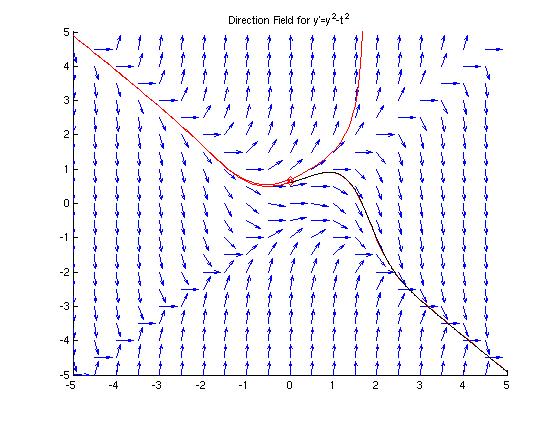
We will use the 'dirfield' module to plot the direction field for this differential equation. As directed in the text, we will also look at the
solution curves with = 0 and = 1. The upper curve corresponds to = 1 and the lower curve corresponds to = 0.
The MATLAB module 'dirfield.m' used to generate the figures below is available here.
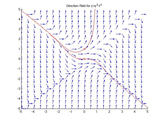
We can "see" the solution with =
0 on the direction field above. It starts
with the two solutions we plotted, then bends up in a somewhat symmetric
rounded "V" shape as t crosses 0.
Our job now is to pinpoint this value of 0
using Euler's method.
The hint in the text is to restrict 0 to an interval of width 0.1. If we use dirfield, we can see that if
= 0.6, the solution curve converges, and if = 0.7
the solution curve diverges. We'll start with this information to try to further pin down the value of 0.
We will start this process with the figure above open, so we can draw our
numerical solution curves to it. (Run 'dirfield' with
y'=y2 - t2, then draw two solution curves with
(t0, y0) = (0, 0.6) and
(t0, y0) = (0, 0.7). Exit dirfield.)
We will implement Euler's method in
MATLAB, repeating it for various values of until we
can get close to the critical value 0.
Recall the formula for Euler's method:
or, equivalently,
 .
.
We will use the second form of Euler's method because it is easier to code into MATLAB and we don't have to be as picky about the indices. (We can't start with a zero entry in a matrix in MATLAB.)
>> clear; % Free memory -- this does not affect the figure
>> diffeq=inline('y^2-t^2','t','y'); % Define function
>> h=0.01; % Set stepsize
>> t0=0; % Set initial t-value
>> y0=0.6; % Set initial y-value
>> t=[0:h:5]; % Make an array of t's from 0 to 5 with stepsize h
>> num=size(t,2); % How many t's do we have?
>> y(1)=y0; % Our first data pt. is (t0,y0)
>> for i=2:num % Loop to implement Euler's method
y(i)=y(i-1)+feval(diffeq,t(i-1),y(i-1))*h; % y(i)=y(1-i)+h*f'(t(i-1),y(i-1))
end
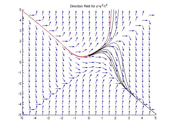
>> plot(t,y,'k'); % Plot results in black on same figure
The graph above seems to be identical to the one from part (a) except that
part of the lower curve is black. The black part is the numerically approximated
solution we found using Euler's method. It's a really good approximation to the curve MATLAB found using it's ODE solver. Now we want to hunt for the value
of 0. We don't need to repeat all of the above
MATLAB commands, we just need to re-define y0, reset y(1), loop to calculate
the y-values, and plot the new result. For example, if we reset y0 to .65:
  >> y0=0.65;
  >> y(1)=y0;
  >> for i=2:num
  y(i)=y(i-1)+feval(diffeq,t(i-1),y(i-1))*h;
  end
  >> plot(t,y,'k');
Below is a graph where this process has been repeated for various values
of y0. The critical value 0 is between the
values of y0 = 0.675 and y0 = 0.68, corresponding to the last curve that converges
and the first one that diverges (bottom to top). The reader can repeat this process to further refine our approximation of 0.