
Find the general solution of the given system of equations. Also draw a direction field and plot a few of the trajectories. In each of these problems, the coefficient matrix has a zero eigenvalue. As a result, the pattern of trajectories is different from those in the examples in the text.
To solve this differential equation, we first need to find the eigenvalues and eigenvectors of the matrix

In MATLAB, this is a simple one-line command, once the matrix has been entered:
  >> A=[3 6;-1 -2];
  >> [V,D]=eig(A)
  V =
      0.9487   -0.8944
     -0.3162    0.4472
  D =
      1.0000         0
           0   -0.0000
  >>
The matrices V and D are the matrices that diagonalize the matrix A. That is, the columns of V are the eigenvectors of A that correspond to the eigenvalues of A found in the corresponding column of the diagonal matrix D. Recall that we can scale the eigenvectors by any value we wish. Thus, for the solution below, I chose to scale the eigenvectors to [3;-1] and [-2;1] to make the formula prettier (but no different). That is, we get eigenvectors and eigenvalues
Using formula (25) in section 7.5 of the text, we find the general solution of the given differential equation is:
or equivalently, as parametric functions,

The MATLAB module dirfield2d.m will plot the direction field of a 2x2 linear system x' = Ax. It also provides the option of plotting individual trajectories on the direction field, when given an user-specified initial point. Here we will run 'dirfield2d' for the matrix A.
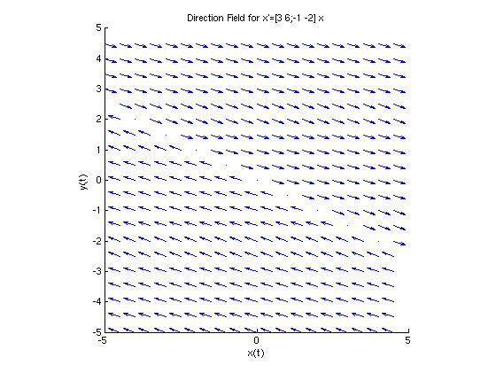
  >> dirfield2d
  Enter the 2x2 matrix A as [a b;c d] => [3 6;-1 -2]

  Enter the window dimensions for the direction field:
     Enter the smallest x value => -5
     Enter the largest  x value => 5
     Enter the smallest y value => -5
     Enter the largest  y value => 5
  Warning: Divide by zero.
  > In dirfield2d at 87
  Warning: Divide by zero.
  > In dirfield2d at 88

  Would you like to plot a solution curve on this direction field? (y or n) => n
  >>
Note: The 'divide by zero' warnings are true (and many more of them occur than are shown here), but we can ignore them. We'll get that warning anywhere the slope line becomes vertical or undefined. For this example, that happens along the line of dots we see in the center of the graph, where the arrows abruptly change direction.
If we answer 'y' instead of 'n' to the last question in dirfield2d, we are prompted to enter the coordinates of an initial condition that determines the integral curve (trajectory) on the direction field that corresponds to the particular solution to the initial value problem.
Here is the phase plot that arises when we plot the 6 trajectories with initial conditions (x(0), y(0)) as shown below:
| (0, -5), | (0, -3), | (0, -1), |
| (0, 1), | (0, 3), | (0, 5). |
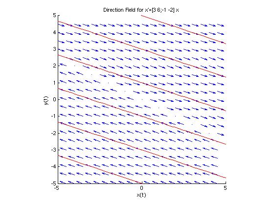
This looks nothing like the examples in the text. In fact, it looks like nothing more interesting than a set of parallel lines. (Which is in itself pretty interesting.) Why? Which line is it and how does it relate to the matrix A? What does that line of dots mean?
Although the solutions x(t) and y(t) both involve exponential functions, there is a simple relationship between them:

Each of these lines is in the direction of the eigenvector v1. However, these lines have a different slope than the line of dots down the center of the graph where the derivatives have no length. Let's look what happens to solutions that intersect that line of dots. That line is y = -x/2, and it's plotted on the graph in aqua after the 'dirfield2d' module is finished.
  >> dirfield2d
  Enter the 2x2 matrix A as [a b;c d] => [3 6;-1 -2]

  Enter the window dimensions for the direction field:
     Enter the smallest x value => -5
     Enter the largest  x value => 5
     Enter the smallest y value => -5
     Enter the largest  y value => 5
  Warning: Divide by zero.
  > In  dirfield2d at 87
  Warning: Divide by zero.
  > In  dirfield2d at 88

  Would you like to plot a solution curve on this direction field? (y or n) => y
  Enter x(0) for this initial value problem => 0
  Enter y(0) for this initial value problem => -.5

  Would you like to plot another solution curve (y or n) => y
  Enter x(0) for this initial value problem => 0
  Enter y(0) for this initial value problem => -.25

  Would you like to plot another solution curve (y or n) => y
  Enter x(0) for this initial value problem => 0
  Enter y(0) for this initial value problem => .25

  Would you like to plot another solution curve (y or n) => y
  Enter x(0) for this initial value problem => 0
  Enter y(0) for this initial value problem => .5

  Would you like to plot another solution curve (y or n) => n
  >> fplot(inline('-t/2','t'),[-5 5],'c--');   % Plot y = x/2 in aqua
  >>
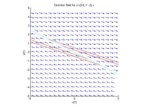
The solutions stop abruptly when they cross the aqua line. Why? Although there is a linear relationship between x and y, they are still defined by exponential functions, and one of the fundamental properties of exponential functions is that they are never negative. Let's consider the case when (x0, y0) = (0, 0.5), which produces the uppermost red line shown on the graph above. The parametric equations for this line are
| x(t) =3et - 3 |
| y(t) =-et + 1.5 |
Thus, for any values of t, we have x(t) > 3 and y(t) < 1.5. The points where these solutions start and stop lie along the line y = -x/2, which is the line through the eigenvector [2;-1] corresponding to the eigenvalue of 0. The derivatives along this line all have value 0, because x' = Ax = 0 for x along this eigenvector line.