Consider the initial value problem
$$ u''+\gamma u'+u=0,\quad u(0)=2,\quad u'(0)=0. $$ We wish to explore how long a time interval is required for the solution
to become "negligible" and how this interval depends on the damping coefficient
$\gamma$. To be more precise, let us seek the time
$\tau$ such that $|u(t)|<0.01$ for all
$t>\tau$. Note that critical damping for this problem
occurs for $\gamma=2$.
(a) Let $\gamma=0.25$ and determine $\tau$, or at least estimate it fairly accurately from a plot of the solution.
(b) Repeat part (a) for several other values of $\gamma$ in the
interval $0<\gamma<1.5$. Note that $\tau$
steadily decreases as $\gamma$ increases for
$\gamma$ in this range.
(c) Create a graph of $\tau$ versus $\gamma$ by plotting the pairs of values found in parts (a) and (b). Is the graph a
smooth curve?
(d) Repeat part (b) for values of $\gamma$ between $1.5$ and $2$. Show that $\tau$ continues to decrease until $\gamma$
reaches a certain critical value $\gamma_0$, after which $\tau$ increases. Find $\gamma_0$ and the corresponding minimum value of $\tau$ to two decimal places.
(e) Another way to proceed is to write the solution of the initial value
problem in the form (26). Neglect the cosine factor and consider only the exponential factor and the amplitude R. Then find an expression for
$\tau$ as a function of $\gamma$. Compare the approximate results obtained in this way with the values determined in parts
(a), (b) and (d).
Since $\gamma=0.25$, we can use the methods of section 3.4 to find the solution of this second order initial value problem. We get:
$$ u(t)=2e^{-\frac18t}\cos\left(\tfrac{3\sqrt{7} t}{8}\right)+\tfrac{2}{3\sqrt{7}}e^{-\frac18t}\sin\left(\tfrac{3\sqrt{7} t}{8}\right). $$The following MATLAB code will generate a graph of this solution curve:
MATLAB note: We need to use the matrix operators '.*' and './' to do multiplication and division term-by-term on arrays. If we forget to use the '.', then MATLAB will try to do standard matrix multiplication and 'division' (multiplication by an inverse), which will fail since the dimensions of these arrays are not compatible. Remember that 'tpts' and 'ypts' are arrays, not single values.
  >> gamma=.25;
  lambda=-gamma/2;               % lambda and mu come from the quadratic formula
  mu=sqrt(4-gamma^2)/2;
  a=2;                           % a and b are the constants in y(t) = a*y1(t) + b*y2(t)
  b=-2*lambda/mu;                %   where y1 and y2 are fundamental solutions
  tmin=0;
  tmax=100;
  stry=sprintf('%g*exp(%g.*t).*cos(%g.*t) + %g*exp(%g.*t).*sin(%g.*t)',a,lambda,mu,b,lambda,mu);
  y=inline(stry,'t');
  figure;                        % Create a figure
  hold on;
  tpts=(tmin:0.001:tmax);        % Generate t-values
  ypts=feval(y,tpts);            % Generate corresponding y-values
  plot(tpts,ypts);               % Plot points
  axis([tmin tmax -1 1]);        % Set window size
  xlabel('t');                   % Identify horizontal axis
  ylabel('u(t)');                % Identify vertical axis
  title(sprintf('Gamma = %g',gamma));     % Add title to identify gamma
  >>
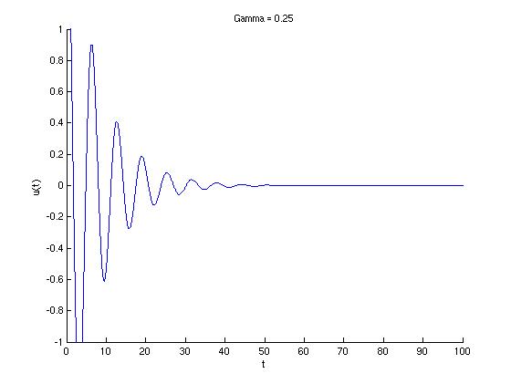
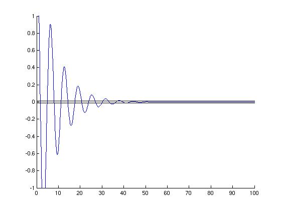
We want to find the value of $\tau$ so that $-0.01< u(t)<0.01$ for all $t>\tau$. That is, we want to find the smallest value of $t$ so that $u(t)$ is between the aqua lines shown on the graph below from that point onward. These commands will add to the graph created above.
  >> tolerance=0.01;
  z=inline(sprintf('%g',tolerance),'t');      % Define the function z = 0.01
  negz=inline(sprintf('%g',tolerance),'t');   % Define the function negz = -0.01
  fplot(z,[tmin,tmax],'c');                   % Plot the horizontal line y = 0.01
  fplot(negz,[tmin,tmax],'c');                % Plot the horizontal line y = -0.01
Instead of looking for the value of $t$ for which all $y$-values beyond that point are between $-0.01$ and $0.01$, let's look backwards from the right side of the graph back to the left. When is the first time the graph of the solution crosses either one of the horizontal aqua lines going from right to left?
  >> num=size(ypts,2);          % How many points did we have?
  for i=1:num
  j=num+1-i;                        % Count backwards
  if abs(ypts(j))>tolerance         % if outside of the aqua lines, notify user
  disp(sprintf('\nFor all t > %g, -%g < y < %g',tpts(j), tolerance, tolerance));
  break            % Exit loop when we find the first y-value outside of the aqua band
  end
  end
  plot(tpts(j),ypts(j),'rp')           % Add a red star
  plot(tpts(j:num),ypts(j:num),'r')    % Re-draw the end of the curve in red

  For all t > 41.715, -0.01 < y < 0.01
  >>
Thus, when $\gamma=0.25$, $\tau= 41.7417$.
Note: This is only an approximation and not an exact value for $\tau$.
If we were to increase the number of points in the arrays 'tpts' and 'ypts' (back in
the 'tpts=(tmin:0.001:tmax)' command, we'd get
a more precise answer for $\tau$. However, we'd also greatly
increase the computation time.
The MATLAB module Ch03Sec07Prob25 will find the value of $\tau$ for a user-entered value of $\gamma$, and allow the user to create the final graph above if desired. This module was used to obtain the data below and in part (d).
If we repeat the above process for values of $\gamma$ between $0$ and $1.5$, we get the values for $\tau$ in the table below:
| $\gamma$ | $\tau$ |
|---|---|
| 0.1 | 104.262 |
| 0.2 | 51.208 |
| 0.25 | 41.715 |
| 0.3 | 35.288 |
| 0.4 | 26.237 |
| 0.5 | 20.402 |
| 0.6 | 17.336 |
| 0.7 | 14.548 |
| 0.8 | 11.845 |
| 0.9 | 11.682 |
| 1.0 | 9.168 |
| 1.1 | 9.226 |
| 1.2 | 9.097 |
| 1.3 | 6.729 |
| 1.4 | 6.989 |
The points from part (b) are plotted in the graph below:
  >> xx=[.1 .2 .25 .3 .4 .5 .6 .7 .8 .9 1 1.1 1.2 1.3 1.4]
  >> yy=[104.262 51.208 41.715 35.288 26.237 20.402 17.336 14.548 11.845 11.682 9.168 9.226 9.097 6.729 6.989];
  >> figure
  >> plot(xx,yy,'bs')            % Plot blue squares this time
  >> xlabel('Gamma');
  >> ylabel('Tau');
  >> title('Tau -vs- Gamma');
  >>
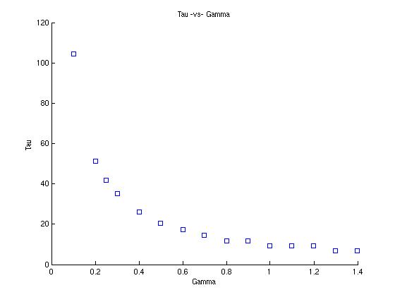
The values appear to decay exponentially, but if we look closely, the numbers do not always decrease.
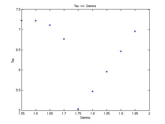
Here is a table of values for $\gamma$ between $1.5$ and $2$ and the corresponding plot:
| $\gamma$ | $\tau$ |
|---|---|
| 1.55 | 7.230 |
| 1.60 | 7.218 |
| 1.65 | 7.108 |
| 1.70 | 6.767 |
| 1.75 | 5.033 |
| 1.80 | 5.472 |
| 1.85 | 5.956 |
| 1.90 | 6.459 |
| 1.95 | 6.956 |
As we can see in the graph below, there is a definite dip in the values of $\tau$ near $1.75$.
  >> xx2=[1.55 1.6 1.65 1.7 1.75 1.8 1.85 1.9 1.95];
  >> yy2=[7.23 7.218 7.108 6.767 5.033 5.472 5.956 6.459 6.956];
  >> plot(xx2,yy2,'bp');
  >> xlabel('Gamma');
  >> ylabel('Tau');
  >> title('Tau -vs- Gamma');
  >>
Now, let's investigate further to find out which value of $\gamma$ produces the lowest value of $\tau$. It appears to be between $1.7$ and $1.8$. Further experimentation gives us the following table:
| $\gamma$ | $\tau$ |
|---|---|
| 1.71 | 6.612 |
| 1.72 | 6.245 |
| 1.73 | 4.873 |
| 1.74 | 4.952 |
| 1.75 | 5.033 |
| 1.76 | 5.117 |
| 1.77 | 5.202 |
| 1.78 | 5.290 |
| 1.79 | 5.380 |
Thus, to two decimal places, the lowest value of $\tau$ is $4.873$ when $\gamma$ is $1.73$.
The form of the solution to the initial value problem is
$$ u(t)=A e^{\lambda t}\cos(\mu t)+ Be^{\lambda t}\sin(\mu t) $$where $\lambda\pm i\mu$ are the roots of the characteristic equation. Using the quadratic formula, we find that $\lambda=-\gamma/2$ and $\mu=\sqrt{4-\gamma^2}/2$.
As functions of $g$, the coefficients $A$ and $B$ are found to be $A=2$ and $B=-\tfrac{\lambda}{\mu}=\tfrac{2\gamma}{\sqrt{4-\gamma^2}}$. If we write $u(t)$ in the form (26), we have
$$ u(t)=Re^{-\gamma t/2}\cos(\mu t-\delta), $$where $A=R\cos\delta$ and $B=R\sin\delta$. Using trigonometry, we find that $\delta=\tan^{-1}\left(\frac\gamma{\sqrt{4-\gamma^2}}\right)$ and subsequently $R=\frac{2}{\cos\left(\tan^{-1}\left(\frac\gamma{\sqrt{4-\gamma^2}}\right)\right)}=\frac{4}{\sqrt{4-\gamma^2}}$.
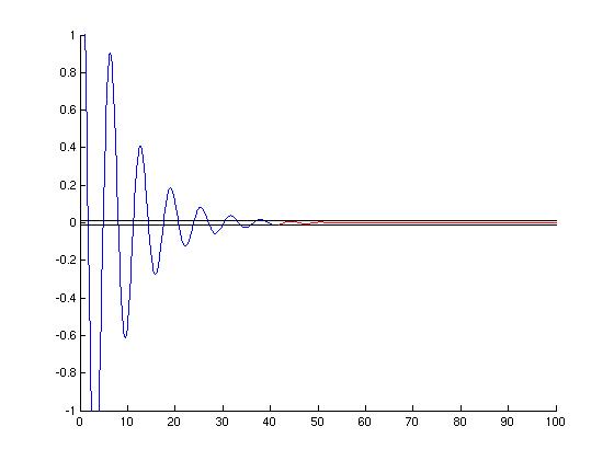
If we ignore the cosine factor, we get the envelope function $U(t)=\frac4{\sqrt{4-\gamma^2}} e^{-\gamma t/2}$. A graph of this function together with the actual solution $u(t)$ is shown below for $\gamma=.25$.
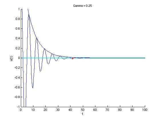
We can see from the graph that $-0.1{}<{}u(t)<0.1$ wherever $U(t)<0.1$. So, let's see where that happens. For simplicity, we will again write the amplitude as $R$. First, we need to solve
$$ Re^{-\gamma\tau/2}=0.01. $$Solving for $\tau$, we have
$$ \tau=-\tfrac{2}{\gamma}\ln(0.1/R)=-\tfrac2\gamma\ln\left(.0025\sqrt{4-\gamma^2}\right)=-\tfrac2\gamma\ln\left(\sqrt{4-\gamma^2}/400\right)=\tfrac2\gamma\ln\left(400/\sqrt{4-\gamma^2}\right). $$Now, we have $\tau$ as a function of $\gamma$. Let's use MATLAB to compare values from this function to our previously found values of $\tau$.
  >> gamma=[.1 .2 .25 .3 .4 .5 .6 .7 .8 .9 1.0 1.1 1.2 1.3 1.4 1.55 1.6 1.65 1.7 1.75 1.8 1.85 1.9 1.95];
  >> T=inline('(2./g).*log(400./sqrt(4-g.*g))','g');     % define tau function
  >> tau=feval(T,gamma)                                  % evaluate tau's
  tau =
    Columns 1 through 9
    105.9914   53.0334   42.4495   35.3980   26.5936   21.3223   17.8182   15.3247   13.4637
    Columns 10 through 18
     12.0255   10.8843    9.9608    9.2024    8.5736    8.0500    7.4287    7.2614    7.1140
    Columns 19 through 24
      6.9874    6.8843    6.8096    6.7740    6.8024    6.9769
  >>
Below is a table that compares the values of $\tau$ using the graphical approximation method and the algebraic approach above.
| $\gamma$ | Approx. $\tau$ from (b) and (d) |
Approx. $\tau$ from (e) |
|---|---|---|
| 0.1 | 104.262 | 105.9914 |
| 0.2 | 51.208 | 53.0334 |
| 0.25 | 41.715 | 42.4495 |
| 0.3 | 35.288 | 35.3980 |
| 0.4 | 26.237 | 26.5936 |
| 0.5 | 20.402 | 21.3223 |
| 0.6 | 17.336 | 17.8182 |
| 0.7 | 14.548 | 15.3247 |
| 0.8 | 11.845 | 13.4637 |
| 0.9 | 11.682 | 12.0255 |
| 1.0 | 9.168 | 10.8843 |
| 1.1 | 9.226 | 9.9608 |
| 1.2 | 9.097 | 9.2024 |
| 1.3 | 6.729 | 8.5736 |
| 1.4 | 6.989 | 8.0500 |
| 1.55 | 7.230 | 7.4287 |
| 1.60 | 7.218 | 7.2614 |
| 1.65 | 7.108 | 7.1140 |
| 1.70 | 6.767 | 6.9874 |
| 1.75 | 5.033 | 6.8843 |
| 1.80 | 5.472 | 6.8096 |
| 1.85 | 5.956 | 6.7740 |
| 1.90 | 6.459 | 6.8024 |
| 1.95 | 6.956 | 6.9769 |
The reason for the difference between the two approximations for $\tau$ is that we ignored the cosine term in part (e). Thus, the two columns should not be exactly alike. However, since the exponential function used in part (e) is always greater than the actual function used in the rest of the problem, we should expect that the values in the second column are always greater than (or equal to) those in the first, which is the case.
Comments: In part (c), we noticed that the graph of $\tau$ versus $\gamma$ appeared to decay exponentially. In part (e), we have found that the equation of this function is not an exponential function, but is instead a more complicated logarithmic function.