For the system
(a) Find the eigenvalues and eigenvectors.
(b) Classify the critical point (0,0) as to type and determine whether
it is stable, asymptotically stable, or unstable.
(c) Sketch several trajectories in the phase plane and also sketch some typical
graphs of x1 versus t.
(d) Use a computer to plot accurately the curves requested in part (c).
MATLAB can easily find the eigenvectors and eigenvalues for this system:
  >> A=[-1 -1;0 -0.25];
  >> [V,D] = eig(A)
  V =
      1.0000   -0.8000
           0    0.6000
  D =
     -1.0000         0
           0   -0.2500
  >>
Thus, we see that the eigenvectors &xi1 and &xi2 and eigenvalues v1 and v2 are:
Both eigenvalues are real and negative. Thus, according to Table 9.1.1 in Section 9.1 of the text, the origin is a node and it is asymptotically stable.
The general solution to this system is
The MATLAB code below will plot 25 curves (not necessarily distinct) for values of c1 and c2 between -2 and 2.
  >> c = [-2 -1 0 1 2];       % These are the coefficients for the solutions
  >> tpts = [-50:0.05:10];
  >> % Open figure, add labels and title
  >> figure; hold on;
  >> xlabel('x_{1}(t)'); ylabel('x_{2}(t)');
  >> title('Phase Portrait for Problem #8 in Section 9.1');
  >> % Loop to use c-values in each slot of general solution
  >> for i = 1:5
  for j = 1:5
  strx1=sprintf('%d*exp(-t) + %d*(-0.8)*exp(-0.25*t)',c(i),c(j));
  strx2=sprintf('%d*(0.6)*exp(-0.25*t)',c(j));
  x1=inline(strx1,'t');
  x2=inline(strx2,'t');
  plot(x1(tpts),x2(tpts));
  end
  end
  >> axis([-2 2 -2 2]);        % Re-size window
  >>
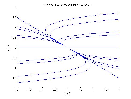
Because the origin is an asymptotically stable node, these trajectories are traversed inward, toward the origin. We can also plot a few representative graphs of x1 versus t.
  >> % Open figure, add labels and title
  >> figure; hold on;
  >> xlabel('t'); ylabel('x_{1}(t)');
  >> title('x_{1}(t) versus t for Problem #8 in Section 9.1');
  >> % These are the coefficients for the 8 curves to graph
  >> c1=[1 1 -1 -1  3 3 -3 -3];
  >> c2=[1 -1 -1 1 1 -1 1 -1];
  >> % Loop to graph the 8 curves
  >> for i = 1:8
  strx1=sprintf('%d*exp(-t) + %d*(-0.8)*exp(-0.25*t)',c1(i),c2(i));
  x1=inline(strx1);
  plot(tpts, x1(tpts));
  end
  >> axis([-10 10 -10 10]);             % Re-size window
  >>
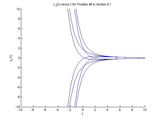
As we expected, each curve approaches 0 as t approaches infinity.