Chapter 9, Section 2, Problem #23

Problem #23

For the differential equation dx/dt = y, dy/dt = -sin(x) that models the motion of an undamped pendulum:

(a) Find an equation of the form H(x,y) = c satisfied by the trajectories.

(b) Plot several level curves of the function H. These are trajectories of the given system. Indicate the direction of motion on each trajectory.

Part (a)

We can solve this problem using separation of variables. We have dy/dx = -sin x/y. Separating variables and integrating both sides, we find the solution is y²/2 - cos x = c, where c is any real constant. Thus,

H(x, y) = y²/2 - cos x,

and solutions are given by H(x, y) = c.

Part (b)

Solutions to this differential equation are easy to plot, because we can solve the equation H(x, y) = c for y:

The module Ch09Sec02Prob23.m creates the figure below, color-coding the three different types of solutions as shown.

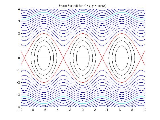
First, we notice from the equation of the solution that the solutions are complex if c < -1. Thus, we only consider values of c &ge -1.

The black curves arise for -1 < c < 1, where the quantity under the radical can become negative, so the solution curves are not defined for all values of x and are thus disconnected. Each value of c < 1 gives an infinite sequence of closed loops. An initial value would specify which of these closed loops solves a particular initial value problem.
The red curve arises from c = 1, where the quantity under the radical is never negative, but might be zero. This curve clearly marks the transition from the disconnected oval solution curves to the oscillating wave solutions.
The blue curves arise from c > 1, where the quantity under the radical is always positive. Each value of c > 1 gives a pair of oscillating blue curves, one from the negative root and one from the positive root. One such pair is illustrated in aqua (when c = 6.0).

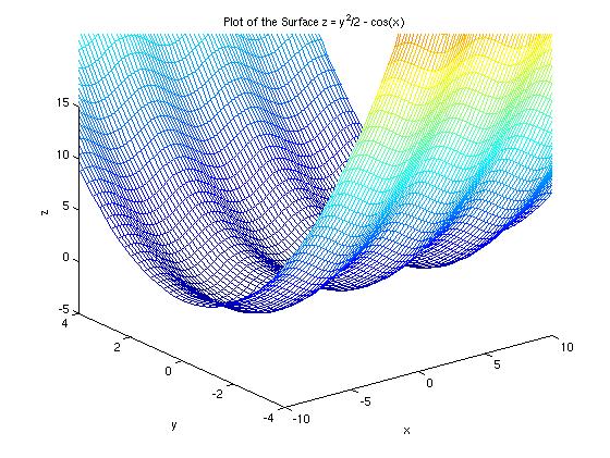
The solution curves to the differential equation are the level curves of the function z = H(x,y). This surface is shown below:

  >> z=inline('y.^2/2-cos(x)','x','y');
  >> figure; hold on;
  >> xlabel('x'); ylabel('y'); zlabel('z');
  >> title('Plot of the Surface z = y^2/2 - cos(x)'); 
  >> % Construct grid for x,y points in the plane
  >> Mrow=[-10:0.25:10];  % Points on each axis 
  >> cols=size(Mrow,2);
  >> M=Mrow';             % First column of M is transpose of Mrow
  >> for i = 1:cols-1     % Creates a square array with all columns Mrow'
  M=[M Mrow'];
  end
  >> xpts=M';             % x-coords of points (i,j) 
  >> ypts=M;              % y-coords of points (i,j) 
  >> zpts=z(xpts,ypts);   % z-coords of points (i,j) 
  >> % This is the command to make a surface plot and show the grid on the surface 
  >> meshc(xpts,ypts,zpts);
  >> view(3);             % Ensure a 3-d view
  >> axis([-10 10 -4 4 -5 15]);    % Resize window

Note: MATLAB has a built-in command to do a contour plot. If we use it, we get the figure below, which does not show all of the details of the plot we created ourselves using module "Ch09Sec02Prob23.m". However, if the solution equation H(x,y) = c was not solvable for y, we would have needed to rely on the built-in function.

  >> % We are assuming that the commands used above to set 'xpts',ypts' 
  >> %     and 'zpts' have already been executed as in the previous example.
  >> figure; hold on;
  >> contour(xpts,ypts,zpts,20)   % Draw 20 contour lines
  >> title('Contour Plot of H(x,y) = y^2/2 - cos(x) using MATLAB command ''contour''');
  >> xlabel('x'); ylabel('y'); 
  >> axis([-10 10 -4 4]);
  >>

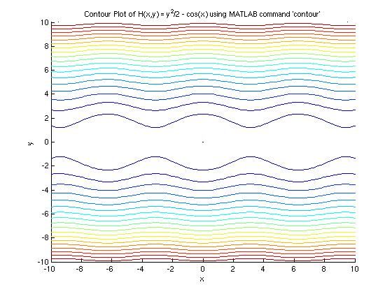
The colors of the contour plot correspond to the height z on the surface. The lowest curves are black, and the colors cycle up to red for the highest curves. However, the colors do not necessarily correspond to the colors used in the surface plot above.