Chapter 9, Section 4, Problem #4

Problem #4

The problem below can be interpreted as describing the interaction of two species with populations x and y.

Carry out the following steps:
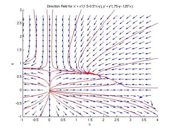
(a) Draw a direction field and describe how the solutions seem to behave.

(b) Find the critical points.

(c) For each critical point find the corresponding linear system. Find the eigenvalues and eigenvectors of the linear system; classify each critical point as to type, and determine whether it is asymptotically stable, stable, or unstable.

(d) Sketch the trajectories in the neighborhood of each critical point.

(e) Compute and plot enough trajectories of the given system to show clearly the behavior of the solutions.

(f) Determine the limiting behavior of x and y as t approaches infinity, and interpret the results in terms of the populations of the two species.

Part (a)

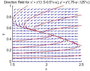
We can use the MATLAB module dirfieldAuto to plot the direction field for this system. The critical points (found in part (b) are marked with red stars.)

  >> dirfieldAuto
  *-----------------------------------------------------------*
  | This module will plot a direction field for an autonomous |
  | system of equations x' = f(x,y), y' = g(x,y).             |
  *-----------------------------------------------------------*
 
    Enter x' as a function of x and y:  x' => x*(1.5-0.5*x-y)
    Enter y' as a function of x and y"  y' => y*(0.75-y-0.125*x)
    Enter the smallest x value => -1
    Enter the largest x value  => 4
    Enter the smallest y value => -1
    Enter the largest y value  => 3
  Warning: Divide by zero.
  > In dirfieldAuto at 88
  Warning: Divide by zero.
  > In dirfieldAuto at 89
  Warning: Divide by zero.
  > In dirfieldAuto at 88
  Warning: Divide by zero.
  > In dirfieldAuto at 89
  >> plot([0 0 2 3],[0 0.75 0.5 0],'rp')  % Plot stars at critical points 
  >>

Part (b)

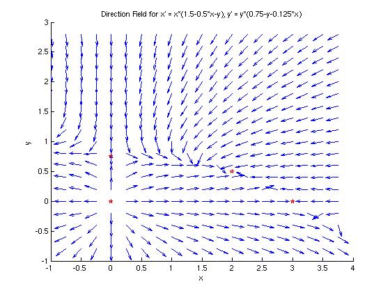
Using basic algebra, we find that the critical points for this system are (0,0), (0, 0.75), (2, 0.5) and (3,0). They are marked with red stars on the direction field in part (a).

Part (c)

Critical Point (0,0)

The linear system that approximates the non-linear system near the critical point (0,0) is

Because the coefficient matrix is diagonal, we can see that the eigenvalues are &xi₁ = 1.5 and &xi₂ = 0.75. The eigenvectors are easily shown to be v₁ = [1;0] and v₂=[0;1]. Because both eigenvalues are real and positive, the origin is an unstable node.

Critical Point (0,0.75)

The linear system that approximates the non-linear system near the critical point (0,0.75) is

The MATLAB command 'eig' will find the eigenvalues of the coefficient matrix:

  >> [V,D]=eig([0.75 0;-0.09375 -0.75])
  V =
           0    0.9981
      1.0000   -0.0624
  D =
     -0.7500         0
           0    0.7500
  >>

Thus, the eigenvectors and eigenvalues of the coefficient matrix are

The eigenvalues are real with opposite sign, so the critical point (0, 0.75) is a saddle point and is unstable.

Critical Point (2,0.5)

The linear system that approximates the non-linear system near the critical point (2,0.5) is

The MATLAB command 'eig' will find the eigenvalues of the coefficient matrix:

  >> [V,D]=eig([-1 -2;-0.0625 -0.5])
  V =
     -0.9958    0.9463
     -0.0911   -0.3232
  D =
     -1.1830         0
           0   -0.3170
  >>

Thus, the eigenvectors and eigenvalues of the coefficient matrix are

The eigenvalues are real, distinct, and negative, so the critical point (2, 0.5) is an asymptotically stable node.

Critical Point (3,0)

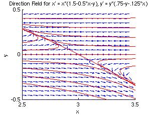
The linear system that approximates the non-linear system near the critical point (3, 0) is

The MATLAB command 'eig' will find the eigenvalues of the coefficient matrix:

  >> [V,D]=eig([-1.5 -3;0 0.375]) 
  V =
      1.0000   -0.8480
           0    0.5300
  D =
     -1.5000         0
           0    0.3750
  >>

Thus, the eigenvectors and eigenvalues of the coefficient matrix are

The eigenvalues are real with opposite sign, so the critical point (3, 0) is a saddle point and is unstable.

Parts (d) and (e)

The 'dirfieldAuto' module will plot solution curves if we choose, which allows us to create a phase portrait on top of a direction field. Here 24 curves are plotted to create the phase portrait.

Let's analyze the behavior of the trajectories near the four critical points:

We can see that all curves lead away from the origin, and those that leave along an axis stay straight. All other curves bend toward the horizontal axis, at least for a while.
The only curves that lead toward the critical points at (0, 0.75) and (3,0) are those that approach along the y-axis or x-axis, respectively; of the all other trajectories lead away from these points. This is consistent with what we know of the behavior of saddle points.
All curves in the first quadrant approach the critical point at (2, 0.5). In fact, if we zoom in around this point, it would look like the case of a node of a linear system (in the sense of Chapter 7).

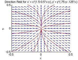
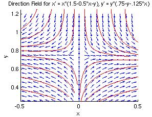
Let's zoom into these four critical points, and look more closely at the phase portraits near them. The four plots below are close-up views of the phase portrait of the non-linear system. Notice how much they look like phase portraits of linear systems.

Critical Point (0, 0)	Critical Point (0, 0.75)
Unstable Node	Unstable Saddle Point

Critical Point (2, 0.5)	Critical Point (3, 0)
Asymptotically Stable Node	Unstable Saddle Point

Part (f)

Because we are considering a population modeled by this system of differential equations, we can assume that x and y are always positive quantities, and thus we only need to consider trajectories in the first quadrant of the coordinate plane. In this quadrant, all trajectories approach the critical point of (2, 0.5), which means that for the populations in question, x will approach 2 and y will approach 0.5, regardless of the initial populations.

In the special cases where one or the other initial population is zero, the trajectories stay on the coordinate axes, and approach one of the critical points (0, 0.75) or (3, 0):

If x(0) = 0, then y will approach 0.75.
If y(0) = 0, then x will approach 3.