The problem below can be interpreted as describing the interaction of two species with population densities x and y.
Carry out the following steps:
(a) Draw a direction field and describe how solutions seem to behave.
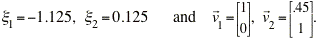
(b) Find the critical points.
(c) For each critical point, find the corresponding linear system. Find the eigenvalues and eigenvectors of the linear system; classify each critical point
as to type, and determine whether it is asymptotically stable, stable, or
unstable.
(d) Sketch the trajectories in the neighborhood of each critical point.
(e) Draw a phase portrait for the system.
(f) Determine the limiting behavior of x and y as t
approaches infinity and interpret the results in terms of the populations of
the two species.
The module dirfieldAuto.m will plot the direction field for a user-specified system. The red stars mark the critical points of the system, and were added after the dirfieldAuto module was run.
>> dirfieldAuto
*-----------------------------------------------------------*
| This module will plot a direction field for an autonomous |
| system of equations x' = f(x,y), y' = g(x,y). |
*-----------------------------------------------------------*
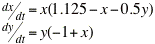
Enter x' as a function of x and y: x' => x*(1.125-x-0.5*y)
Enter y' as a fuhction of x and y" y' => y*(-1+x)
Enter the smallest x value => -0.5
Enter the largest x value => 1.5
Enter the smallest y value => -0.5
Enter the largest y value => 1.5
Warning: Divide by zero.
> In dirfieldAuto at 88
Warning: Divide by zero.
> In dirfieldAuto at 89
>> Would you like to plot a solution curve on this direction field? (y or n) => n
>> plot([0 1 1.125],[0 0.25 0],'rp');
>>
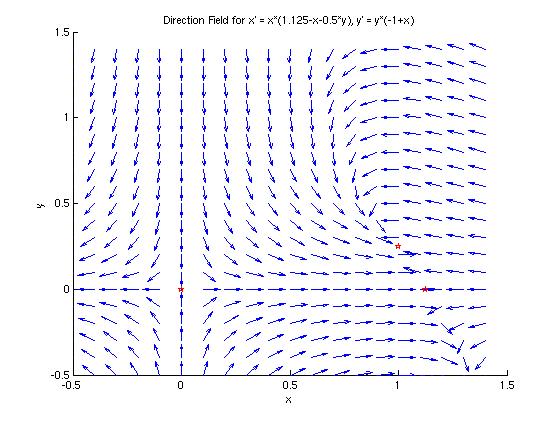
Using basic algebra, we find that the critical points of this system are (0,0), (1,0.25), (1.125,0). These points are marked with red stars on the direction field in part (a).
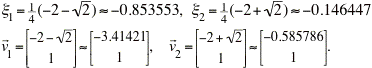
Using formula (13) from Section 9.3, we find that the linear system corresponding to the almost linear system at (0,0) is given by the matrix equation
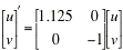
The eigenvalues and eigenvectors for this linear system are:
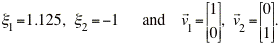
The eigenvalues are real and have opposite signs, so the origin is a saddle point and is thus unstable.
The almost linear system at (1.125, 0) is given by the matrix equation
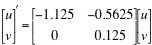
The corresponding eigenvalues for this linear system are:
The eigenvalues are real and have opposite signs, so this point is also a saddle point and is unstable.
Again using formula (13) from Section 9.3, we see that linear system that approximates the almost linear system at the critical point (1, 0.25) is:
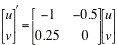
This linear system has eigenvalues and eigenvectors:
The eigenvalues for this linear system are both negative and are unequal, so the point (1, 0.25) is an asymptotically stable node.
The 'dirfieldAuto' module will plot as many trajectories as desired on top of the direction field. They can be slow to plot so be patient.
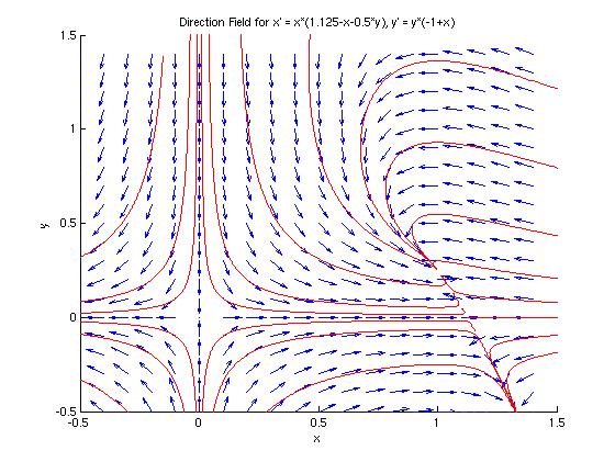
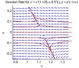
In the plot above, we can clearly see the saddle point behavior at the origin. The saddle behavior at (1.125, 0) is not as apparent, but we can see the trajectories approaching from the left and right then leaving along a diagonal path, as with a saddle point. The spiral behavior at (1, 0.25) is also not perfectly clear from the full direction field. In the figures below, we can zoom in to see the behavior near the critical points at (1.125, 0) and (1, 0.25).
| Critical Point (1.125, 0) |
Critical Point (1, 0.25) |
|---|---|
 |
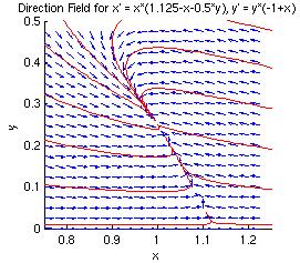 |
In the figure on the left above, we can clearly see that the direction field shows the behavior of a saddle point near (1.125, 0). And, while the figure on the right does look somewhat like a node, it is not a perfect example of one, especially in the upper left corner. If we were to zoom in further, it would look more "node-like".
Since we are studying two populations, we can assume that x &ge 0 and y &ge 0. Thus, we are only concerned with the first quadrant of the phase portrait above. From the phase portrait, and from what we know about the linear systems that approximate the non-linear system near the critical points, we can see that there are only three long-term possibilities for these two populations.