For the Van der Pol equation,
(a) Find all the critical points (equilibrium solutions).
(b) Use a computer to draw a direction field and phase portrait for the
system.
(c) From the plot(s) in part (b), determine whether each critical point is
asymptotically stable, stable, or unstable, and classify it as to type.
By solving x' = 0 and y' = 0, we find that the only critical point of this system is (0, 0).
The module dirfieldAuto.m will plot a direction field for any autonomous system (meaning, without explicit use of 't') of two equations in x and y and gives the user the option to plot solution curves to initial value problems. The difference between this module and 'dirfield2d' is that 'dirfield2d' solves linear systems exactly, where 'dirfieldAuto' uses one of MATLAB's built-in ODE solvers to calculate a solution. It is slower and less exact than dirfield2d, but for non-linear systems it's the best we can do.
  >> dirfieldAuto
  *-----------------------------------------------------------*
  | This module will plot a direction field for an autonomous |
  | system of equations x' = f(x,y), y' = g(x,y).             |
  *-----------------------------------------------------------*

    Enter x' as a function of x and y:  x' => y
    Enter y' as a function of x and y:  y' => (1-x^2)*y-x
    Enter the smallest x value => -3
    Enter the largest x value  => 3
    Enter the smallest y value => -3
    Enter the largest y value  => 3
  Warning: Divide by zero.
  > In dirfieldAuto at 86
  Warning: Divide by zero.
  > In dirfieldAuto at 87
  >> Would you like to plot a solution curve on this direction field? (y or n) => n
  >>
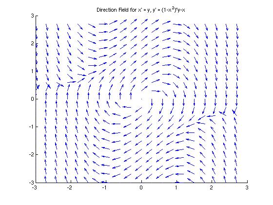
Looking at the direction field, it seems that the origin is an unstable critical point, as it appears that the trajectories all leave the origin in a spiraling motion. However, we'll need to look at some actual trajectories to be sure that this is the case.
Now, we can run 'dirfieldAuto' again, answering 'y' to the final question to plot some trajectories. the figure below was created using 8 sets of initial conditions.
Warning: This module takes awhile to calculate solutions. Be patient.
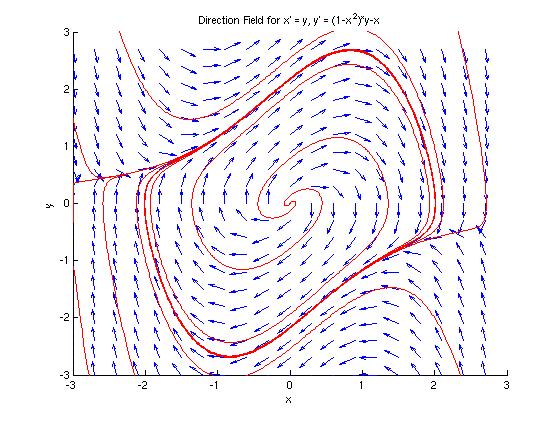
From the plot in part (b), we see that the origin is an unstable critical point. In fact, all trajectories approach the pillow-shaped closed curve shown on the phase portrait, whether they start inside or outside of that curve.