Problem #18

(a) Find the solution u(t) for

(b) Plot the solution u(t) versus t for , , and . Describe how the response u(t) changes as varies in this interval. What happens as takes on values closer and closer to 1? Note that the natural frequency of the unforced system is .

Part (a)

The solution to this initial value problem for must be found by hand or by using technology with symbolic manipulation capabilities. Here is the solution:

Part (b)

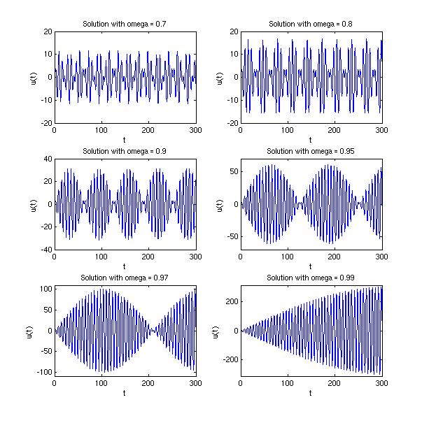
The MATLAB module Ch03Sec09Prob18.m plots one solution to this initial value problem for a value of specified by the user. For brevity, six of these plots are shown together below, created by the following MATLAB code.

  >> tmin=0;
  >> tmax=300;
  >> figure
  >> hold on
  >> omega=[.7 .8 .9 .95 .97 .99];          % we'll plot one solution for each of these values
  >> for i=1:6                              % Loop -- repeat once for each omega
  ustr=sprintf('3/(1-%g^2)*(cos(%g*t)-cos(t))',omega(i),omega(i));
  u=inline(ustr,'t');
  subplot(3,2,i)                 % selects plot i of a 3x2 grid of plots 
  fplot(u,[0,tmax])              % plot solution curve
  amp=abs(6/(1-omega(i)^2));     % determine height of plot based on
  ymax=10*(ceil(amp/10));        %    amplitude of graph
  axis([tmin tmax -ymax ymax]);
  xlabel('t')                    % label axes and plot
  ylabel('u(t)')                
  title(sprintf('Solution with omega = %g',omega(i)));
  end
  >>

.

Notice that in all six of these graphs, the horizontal scale is the same, although the vertical scale changes from figure to figure. We can see from this set of graphs that as approaches 1, the period of the envelope function (what we see as 'pulses') increases. The amplitude of the envelope function increases as well.
(Note: In the last figure, the graph does have 'pulses', the period is just longer than the 300 units allowed by the graphing window.)

Further questions to explore: What happens if = 1? What happens for values of greater than 1?