
Find the solution of the given initial value problem. Draw the trajectory of the solution in the x1x2-plane and also draw the graph of x1 versus t.
We can use MATLAB to do the individual calculations, but we need to find the generalized eigenvector 'eta' step-by-step.
  >> A = [-5/2 3/2;-3/2 1/2]; x0=[3;2];   % Define A and initial condition vector x0
  >> [V,D]=eig(A)
  V =
      0.7071   -0.7071
      0.7071   -0.7071
  D =
     -1.0000         0
           0   -1.0000
  >> L=D(1,1);              % L is the repeated eigenvalue.
  >> v=[V(1,1);V(2,1)];     % v is the repeated eigenvector.
  >> % 'eye(2)' is the 2x2 identity matrix.
  >> B=rref([A-L*eye(2) v])    % Solve this system manually to find eta.
  B =
      1.0000   -1.0000   -0.4714
           0         0         0
  >> eta=[B(1,3);0];           % Found by inspection of B.
  >> % Solution is X(t)=c1*exp(Lt)*v + c2*exp(Lt)*(tv + eta)
  >> coeffs=[v eta]\x0;
  >> c1=coeffs(1); c2=coeffs(2);
  >> % We now know all pieces of X(t). Use '.*' for multiplication.
  >> strx1=sprintf('%g*exp(%g*t)*%g + %g*exp(%g*t).*(t*%g+%g)', c1,L,v(1),c2,L,v(1),eta(1));
  >> strx2=sprintf('%g*exp(%g*t)*%g + %g*exp(%g*t).*(t*%g+%g)', c1,L,v(2),c2,L,v(2),eta(2));
  >> % Convert from strings to functions.
  >> x1 = inline(strx1,'t'); x2 = inline(strx2,'t');
  >> disp(x1)         % Here are the solutions.
       Inline function:
       x1(t) = 2.82843*exp(-1*t)*0.707107 + -2.12132*exp(-1*t)*(t*0.707107+-0.471405)
  >> disp(x2)
       Inline function:
       x2(t) = 2.82843*exp(-1*t)*0.707107 + -2.12132*exp(-1*t)*(t*0.707107+0)
  >>
Now we know that the component functions of the solution are
Let's look at a parametric plot of the trajectory in the x1x2-plane:
  >> tpts=-10:0.01:10;                      % Define t-values
  >> figure; hold on;
  >> plot(x1(tpts),x2(tpts));               % Plot parametrically.
  >> xlabel('x_{1}(t)'); ylabel('x_{2}(t)');
  >> title('x_{2}(t) -vs- x_{1}(t)');
  >> axis([-.5 2 -.5 2]);                   % Resize window to show details.
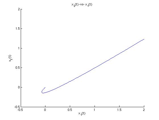
We see deduce that this trajectory is moving toward the origin because the exponential functions are decaying. Let's look now at a graph of x1 -vs- t and see how the two graphs relate.
  >> figure; hold on;
  >> plot(tpts,x1(tpts));     % Plot x1(t) -vs- t
  >> xlabel('t'); ylabel('x_{1}(t)'); title('x_{1}(t) -vs- t');
  >> axis([0 10 -.5 2]);      % Resize window to see details.
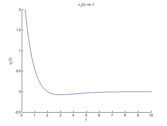
We can estimate the the bottom of the "hook" in the graph of solution curve occurs around t = 3 from looking at the minimum point of the graph of x1. So, as we can see from reading both graphs together, x1 decreases rapidly as t goes from negative infinity to about 3, then x1 increases again (but quite slowly) to 0 as t goes from about 3 to positive inifinity. We can intuit the direction of motion from either graph, but only the graph of x1 -vs- t gives us a sense of how quickly the motion occurs.