
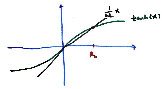
Graphical solution for $\tanh(X) = \frac{1}{hL} X$.
In heat, wave, and Laplace's equations, we repeatedly encountered the ordinary differential equation (ODE):
$$X'' + \lambda X = 0$$
Boundary Conditions: $X(0) = X(L) = 0$ (Ends at fixed temperature)
Boundary Conditions: $X'(0) = X'(L) = 0$ (Ends are insulated)
Both cases gave eigenvalues that are **nonnegative** and form an **increasing sequence**: $\lambda_1 < \lambda_2 < \lambda_3 < \dots$
The eigenfunctions (one for each eigenvalue) are **mutually orthogonal**:
$$\int_0^L X_n X_m dx = 0 \quad \text{if } n \neq m$$
What if we change the BC's, for example:
Or instead of $u_t = k u_{xx}$ (constant conductivity), we use a heat equation where conductivity is a **function of position**?
The general form of a Sturm-Liouville ODE is:
$$\frac{d}{dx}\left[p(x)\frac{dy}{dx}\right] - q(x)y + \lambda r(x)y = 0$$
The Boundary Conditions (BC's) are of the general homogeneous form for $a < x < b$:
At $x=a$: $$\alpha_1 y(a) - \alpha_2 y'(a) = 0$$
At $x=b$: $$\beta_1 y(b) + \beta_2 y'(b) = 0$$
**Constraint:** Not both $\alpha_1$ and $\alpha_2$ can be zero; not both $\beta_1$ and $\beta_2$ can be zero.
The SL problem is said to be **regular** if:
If $q(x)$, $\alpha_1$, $\alpha_2$, $\beta_1$, and $\beta_2$ are all **nonnegative**, then:
ODE: $$y'' + \lambda y = 0 \quad \text{for } 0 < x < L$$
BC's: $y(0) = 0$ and $y(L) = 0$
This ODE can be mapped to the general SL form with: $p(x)=1$, $q(x)=0$, $r(x)=1$.
The BC's map to: $\alpha_1=1, \alpha_2=0$ (at $x=0$) and $\beta_1=1, \beta_2=0$ (at $x=L$).
Since $p, q, r$ are continuous, $p>0$, $r>0$, and all coefficients ($\alpha_1, \alpha_2, \beta_1, \beta_2, q$) are nonnegative, this is a **regular SL problem**.
It agrees with the known heat equation solution: $$\lambda_n = \frac{n^2 \pi^2}{L^2}, \quad y_n = \sin\left(\frac{n\pi x}{L}\right)$$
Properties: $\lambda_1 < \lambda_2 < \dots$ and $\int_0^L y_i y_j dx = 0$ (since $r(x)=1$).
ODE: $$y'' + \lambda y = 0 \quad \text{for } 0 < x < L$$
BC's: $y(0) + y'(0) = 0$ and $y(L) = 0$
At $x=0$: $y(0) + y'(0) = 0 \implies \alpha_1=1, \alpha_2=-1$. Since $\alpha_2$ is negative, this problem is **not guaranteed to have nonnegative eigenvalues**.
This is **not a regular** SL problem because not all $\alpha_1, \alpha_2, \beta_1, \beta_2$ are nonnegative.
ODE: $$y'' + \lambda y = 0$$
BC's: $y(0) = 0$ ($\alpha_1=1, \alpha_2=0$) and $h y(L) - y'(L) = 0$ (where $h>0$).
At $x=L$: $h y(L) - y'(L) = 0 \implies \beta_1=h, \beta_2=-1$. Since $\beta_2 < 0$, this is **not a regular** SL problem, and a negative eigenvalue could exist.
Since the problem is not regular, we start by looking for negative eigenvalues. Let $\lambda = -k^2$, where $k$ is a positive constant ($k>0$).
The ODE becomes: $$y'' - k^2 y = 0$$
General Solution: $y = d_1 \cosh(kx) + d_2 \sinh(kx)$ (more convenient for BC's).
1. Apply $y(0) = 0$:
$$0 = d_1 \cosh(0) + d_2 \sinh(0) \implies 0 = d_1(1) + d_2(0) \implies d_1 = 0$$Solution simplifies to: $y = d_2 \sinh(kx)$, and its derivative is $y' = k d_2 \cosh(kx)$.
2. Apply $h y(L) - y'(L) = 0$:
$$h [d_2 \sinh(kL)] - [k d_2 \cosh(kL)] = 0$$Since the eigenfunction cannot be trivial (i.e., $d_2 \neq 0$), we can divide by $d_2$:
$$h \sinh(kL) = k \cosh(kL)$$Divide by $\cosh(kL)$ (since $\cosh(x)$ is never zero):
$$\tanh(kL) = \frac{k}{h}$$Let $X = kL$. The equation becomes a transcendental equation:
$$\tanh(X) = \frac{X}{hL}$$We solve $\tanh(X) = \frac{1}{hL} X$. This is the intersection of the $\tanh(X)$ curve and a line with positive slope $\frac{1}{hL}$ through the origin.
Let $\beta_0$ be the **smallest positive intersection** of the two graphs.
$$X = \beta_0 = kL \implies k = \frac{\beta_0}{L}$$The **smallest eigenvalue** (which is negative) is:
$$\lambda_0 = -k^2 = -\frac{\beta_0^2}{L^2}$$If $\frac{1}{hL}$ is close to $1$ (the maximum slope $\tanh(X)$ can have at the origin), then $\beta_0 \approx hL$, so $k \approx h$. This gives an approximation for the smallest eigenvalue:
$$\lambda_0 \approx -h^2$$The associated eigenfunction is $y = d_2 \sinh(kx)$. Setting $d_2=1$ for a simplified form gives:
$$\text{Eigenfunction for } \lambda_0: y_0 = \sinh(k_0 x) \quad \text{where } k_0 = \frac{\beta_0}{L}$$This process is the first step. Next, one would find the remaining eigenvalues ($\lambda > 0$), collect all eigenfunctions, and form a solution that will resemble a Fourier-like series.
End of Lesson 34 notes.