Lesson 34: 7.5 Homogeneous Systems with Constant Coefficients

Introduction: Solving Systems

The lesson focuses on solving vector systems in the form $\vec{x}^{\prime}=A\vec{x}$ where the vector is defined as $\vec{x} = \begin{bmatrix}x_{1}\\ \dots \\ x_{n}\end{bmatrix}$. The matrix $A$ consists of constant coefficients.

The solution method is very similar to the scalar example $x^{\prime}=ax$ (or $y^{\prime}=ay$), where the solution involves exponential functions.

Review: Second Order Linear Equation

Consider the scalar equation:

y^{\prime\prime}+5y^{\prime}+6y=0

With initial conditions $y(0)=1$ and $y^{\prime}(0)=2$.

Step 1: Characteristic Equation
We solve using the characteristic polynomial: $r^{2}+5r+6=0$.
Factoring yields: $(r+2)(r+3)=0$, resulting in roots $r=-2, -3$.

The general solution is of the form $x=ce^{at}$ (or in this case for y): $$y=c_{1}e^{-2t}+c_{2}e^{-3t}$$

Using the initial condition $y(0)=1$:

1=c_{1}+c_{2}

Using the derivative $y^{\prime}=-2c_{1}e^{-2t}-3c_{2}e^{-3t}$ and initial condition $y^{\prime}(0)=2$:

2=-2c_{1}-3c_{2}

Converting to a System of First-Order Equations

We can turn the previous example into a system of two 1st-order equations.

Let $x_{1}=y$
Let $x_{2}=y^{\prime}$

This leads to the system:

$x_{1}^{\prime}=x_{2}$ (by definition)
$x_{2}^{\prime}=-6x_{1}-5x_{2}$ (derived from $y^{\prime\prime}=-6y-5y^{\prime}$)

Written in matrix form $\vec{x}^{\prime} = A\vec{x}$:

\begin{bmatrix}x_{1}^{\prime}\\ x_{2}^{\prime}\end{bmatrix}=\begin{bmatrix}0&1\\ -6&-5\end{bmatrix}\begin{bmatrix}x_{1}\\ x_{2}\end{bmatrix}

This is equivalent to $y^{\prime\prime}+5y^{\prime}+6y=0$. The solution corresponds to the scalar solution found earlier:

$x_{1}=y=c_{1}e^{-2t}+c_{2}e^{-3t}$
$x_{2}=y^{\prime}=-2c_{1}e^{-2t}-3c_{2}e^{-3t}$

In vector notation, the solution is:

\begin{bmatrix}x_{1}\\ x_{2}\end{bmatrix}=c_{1}e^{-2t}\begin{bmatrix}1\\ -2\end{bmatrix}+c_{2}e^{-3t}\begin{bmatrix}1\\ -3\end{bmatrix}

The exponents (-2 and -3) are the roots of the characteristic equation. The vectors $\begin{bmatrix}1\\-2\end{bmatrix}$ and $\begin{bmatrix}1\\-3\end{bmatrix}$ must be related to the matrix $A=\begin{bmatrix}0&1\\ -6&-5\end{bmatrix}$.

Eigenvalues and Eigenvectors

The vectors identified above are eigenvectors associated with the eigenvalues $\lambda=-2$ and $\lambda=-3$.

Finding Eigenvalues

To find the eigenvalues, we solve $\det(A-\lambda I)=0$:

\begin{vmatrix}-\lambda&1\\ -6&-5-\lambda\end{vmatrix}=0$$ $$(-\lambda)(-5-\lambda) - (-6)(1) = 0 \rightarrow \lambda^{2}+5\lambda+6=0

This characteristic equation yields roots $\lambda=-2$ and $\lambda=-3$.

Finding Eigenvectors

We solve $(A-\lambda I)\vec{v}=\vec{0}$.

Case 1: $\lambda = -2$ $$A - (-2)I = \begin{bmatrix}2&1\\ -6&-3\end{bmatrix} \rightarrow \begin{bmatrix}2&1\\ 0&0\end{bmatrix}$$ Equation: $2x_1 + x_2 = 0 \rightarrow x_2 = -2x_1$. Eigenvector: $\vec{v}=\begin{bmatrix}1\\ -2\end{bmatrix}$.

Case 2: $\lambda = -3$ $$A - (-3)I = \begin{bmatrix}3&1\\ -6&-2\end{bmatrix} \rightarrow \begin{bmatrix}3&1\\ 0&0\end{bmatrix}$$ Eigenvector: $\vec{v}=\begin{bmatrix}1\\ -3\end{bmatrix}$.

General Solution and Phase Diagrams

The general solution of $\vec{x}^{\prime}=A\vec{x}$ is given by:

\vec{x}=c_{1}e^{\lambda_{1}t}\vec{v}_{1}+c_{2}e^{\lambda_{2}t}\vec{v}_{2}+\dots+c_{n}e^{\lambda_{n}t}\vec{v}_{n}

For our specific example:

\vec{x}=c_{1}e^{-2t}\begin{bmatrix}1\\ -2\end{bmatrix}+c_{2}e^{-3t}\begin{bmatrix}1\\ -3\end{bmatrix}

Phase Diagram (Phase Portrait)

While we can graph $x_1(t)$ and $x_2(t)$ individually, we often get more information from a graph of $x_1$ vs $x_2$. This is called a phase diagram (similar to a slope field).

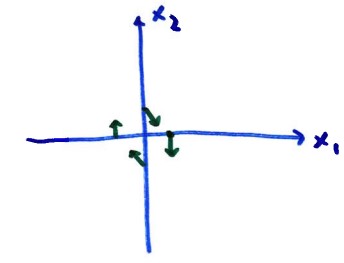
Using $\vec{x}^{\prime}=\begin{bmatrix}0&1\\ -6&-5\end{bmatrix}\vec{x}$, we can calculate tangent vectors at specific points:

At $\vec{x}=\begin{bmatrix}1\\ 0\end{bmatrix}$, $\vec{x}^{\prime}=\begin{bmatrix}0\\ -6\end{bmatrix}$ (Arrow points downward).
At $\vec{x}=\begin{bmatrix}0\\ 1\end{bmatrix}$, $\vec{x}^{\prime}=\begin{bmatrix}1\\ -5\end{bmatrix}$.

Vector field plot showing slopes at various locations. Arrows indicate the direction of flow based on the matrix transformation.

Qualitative Sketch: Nodal Sink

It is easy to sketch qualitatively using the general solution.

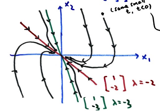
Diagram of Phase Portrait: Origin as Nodal Sink with eigenvectors plotted. Trajectories move inwards toward the origin.

Figure Description: Phase diagram sketch for a Nodal Sink. The origin is the center. Two lines pass through the origin corresponding to eigenvectors v1 (1, -2) and v2 (1, -3). Arrows on all trajectories point inward toward the origin. Trajectories tangentially approach the line of the eigenvector associated with the eigenvalue closest to zero (-2).

As $t \to \infty$, $\vec{x} \to \vec{0}$ (the origin). Solutions go to the origin as $t$ increases.
If $t$ is a large positive number, $e^{-2t}$ is significantly larger than $e^{-3t}$ (since -2 is closer to 0 than -3). Therefore, solutions approach the origin along the eigenvector attached to $\lambda=-2$.
If $t$ is a large negative number, $e^{-3t}$ dominates $e^{-2t}$. Solutions coming from infinity are parallel to the eigenvector for $\lambda=-3$.

Solutions that start exactly on the eigenvector lines remain on those lines, moving toward the origin over time. Generally, trajectories initially follow the direction of the "stronger" (more negative) eigenvalue vector, then curve to follow the "weaker" (less negative) eigenvalue vector on the way to the origin.

Classification: The origin here is called a Nodal Sink because trajectories are attracted to it.

Nodal Source and Saddle Points

If both eigenvalues are positive, the qualitative picture is the same, but the arrows point in the opposite direction (away from the origin). The origin is a Nodal Source.

Example: Saddle Point

Consider $\vec{x}^{\prime}=\begin{bmatrix}1&2\\ 2&1\end{bmatrix}\vec{x}$.

Eigenvalues: $\lambda_1 = -1$ and $\lambda_2 = 3$.
Eigenvectors: $\vec{v}_1 = \begin{bmatrix}1\\ -1\end{bmatrix}$ (for -1) and $\vec{v}_2 = \begin{bmatrix}1\\ 1\end{bmatrix}$ (for 3).
General Solution: $\vec{x}=c_{1}e^{-t}\begin{bmatrix}1\\ -1\end{bmatrix}+c_{2}e^{3t}\begin{bmatrix}1\\ 1\end{bmatrix}$.

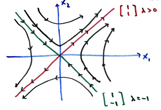
Diagram of Phase Portrait: Origin as Saddle Point. Some trajectories move in, others move out.

Figure Description: Phase diagram of a Saddle Point. The origin is the center. One eigenvector line (1, -1) has arrows pointing IN toward the origin. The other eigenvector line (1, 1) has arrows pointing OUT away from the origin. Trajectories form hyperbolas approaching the origin along the stable eigenvector and curving away along the unstable eigenvector.

The solution $\vec{x}$ never reaches the origin unless we start exactly on the eigenvector associated with the negative eigenvalue ($\lambda=-1$). Because the eigenvalues have opposite signs (one positive, one negative), the origin is classified as a Saddle Point. Trajectories approach along the line of the negative eigenvalue and move away along the line of the positive eigenvalue.