Section 7.8 (continued)
From last time, we were looking at the system:
$$\vec{x}^{\prime}=\begin{pmatrix}1&1\\ 0&1\end{pmatrix}\vec{x}$$
The
matrix has repeated eigenvalues $\lambda=1, 1$. However, we were
missing one eigenvector, as the only true eigenvector found was
$\vec{v}=\begin{pmatrix}1\\ 0\end{pmatrix}$.
The first solution is:
$$\vec{x}^{(1)}=e^{\lambda t}\vec{v}=e^{t}\begin{pmatrix}1\\ 0\end{pmatrix}$$
Revisiting
the scalar case for comparison, the equation
$y^{\prime\prime}+2y^{\prime}+y=0$ has a characteristic equation
$r^2+2r+1=0$ with repeated roots $r=-1, -1$. The general solution is
$y=c_{1}e^{-t}+c_{2}te^{-t}$.
Attempting a
similar approach for the system, let's try
$\vec{x}^{(2)}=te^{t}\begin{pmatrix}1\\ 0\end{pmatrix}$. Substituting
this into $\vec{x}^{\prime}=A\vec{x}$ gives:
$$\vec{x}^{\prime}=(te^{t}+e^{t})\begin{pmatrix}1\\
0\end{pmatrix}=\begin{pmatrix}te^{t}+e^{t}\\ 0\end{pmatrix}$$
$$\mathbf{A}\vec{x}=\begin{pmatrix}1&1\\
0&1\end{pmatrix}\begin{pmatrix}te^{t}\\
0\end{pmatrix}=\begin{pmatrix}te^{t}\\ 0\end{pmatrix}$$
Since $\begin{pmatrix}te^{t}+e^{t}\\
0\end{pmatrix} \ne \begin{pmatrix}te^{t}\\ 0\end{pmatrix}$, the trial
solution $\vec{x}^{(2)}=t\vec{x}^{(1)}$ does not work.
Finding the Second Solution
To
find the second linearly independent solution for
$\vec{x}^{\prime}=A\vec{x}$ when there is a repeated eigenvalue but
only one eigenvector $\vec{v}$, we seek a solution of the form:
$$\vec{x}^{(2)}=te^{\lambda t}\vec{v}+\vec{u}e^{\lambda t}$$
Plugging
this into $\vec{x}^{\prime}=A\vec{x}$ and equating the coefficients of
$te^{\lambda t}$ and $e^{\lambda t}$ yields two equations:
The
vector $\vec{u}$ is called a **generalized eigenvector**. It gets
mapped to the true eigenvector $\vec{v}$ by the matrix $(A-\lambda I)$.
Applying to the Example
Returning
to $\vec{x}^{\prime}=\begin{pmatrix}1&1\\
0&1\end{pmatrix}\vec{x}$, we have $\lambda=1$ and
$\vec{v}=\begin{pmatrix}1\\ 0\end{pmatrix}$.
The first solution is $\vec{x}^{(1)}=e^{t}\begin{pmatrix}1\\ 0\end{pmatrix}$.
The
second solution is $\vec{x}^{(2)}=te^{t}\begin{pmatrix}1\\
0\end{pmatrix}+e^{t}\vec{u}$, where $\vec{u}$ satisfies $(A-\lambda
I)\vec{u}=\vec{v}$.
Substituting the values:
$$\left(\begin{pmatrix}1&1\\
0&1\end{pmatrix}-1\begin{pmatrix}1&0\\
0&1\end{pmatrix}\right)\vec{u}=\begin{pmatrix}1\\ 0\end{pmatrix}$$
$$\begin{pmatrix}0&1\\
0&0\end{pmatrix}\vec{u}=\begin{pmatrix}1\\ 0\end{pmatrix}$$
Let $\vec{u}=\begin{pmatrix}u_1\\
u_2\end{pmatrix}$. This system is $u_2=1$ and $0=0$. We can choose any
value for $u_1$. Choosing $u_1=0$, we get the generalized eigenvector
$\vec{u}=\begin{pmatrix}0\\ 1\end{pmatrix}$.
The second solution is then:
$$\vec{x}^{(2)}=te^{t}\begin{pmatrix}1\\ 0\end{pmatrix}+e^{t}\begin{pmatrix}0\\ 1\end{pmatrix}$$
The **general solution** is:
$$\vec{x}=c_{1}e^{t}\begin{pmatrix}1\\
0\end{pmatrix}+c_{2}e^{t}\left(t\begin{pmatrix}1\\
0\end{pmatrix}+\begin{pmatrix}0\\ 1\end{pmatrix}\right)$$
In component form, this is
$\begin{pmatrix}x_{1}\\
x_{2}\end{pmatrix}=\begin{pmatrix}c_{1}e^{t}+c_{2}te^{t}\\
c_{2}e^{t}\end{pmatrix}$.
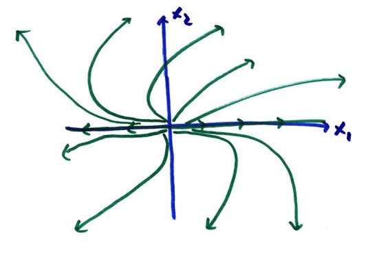
As $t\to\infty$,
both $x_1$ and $x_2$ go to $\infty$ (except for the trivial solution
$c_1=c_2=0$). Solutions go to $\infty$ without following any particular
straight line. However, they approach the origin as $t\to-\infty$.
The ratio of the components as $t\to-\infty$ is:
$$\lim_{t\rightarrow-\infty}\frac{x_{2}}{x_{1}}=\lim_{t\rightarrow-\infty}\frac{c_{2}e^{t}}{c_{1}e^{t}+c_{2}te^{t}}=\lim_{t\rightarrow-\infty}\frac{c_{2}}{c_{1}+c_{2}t}=0$$
This shows that solutions approach the
origin along the line $x_2=0$, which is the line corresponding to the
true eigenvector. This true eigenvector is a line of zero slope. The
phase portrait shows this behavior (solutions go to the origin along
the true eigenvector, making the generalized eigenvector "invisible" in
terms of direction).
Section 7.7 Fundamental Matrix
Consider
a system $\vec{x}^{\prime}=A\vec{x}$ whose two linearly independent
solutions are $\vec{x}^{(1)}=e^{2t}\begin{pmatrix}2\\ 1\end{pmatrix}$
and $\vec{x}^{(2)}=e^{-t}\begin{pmatrix}1\\ 2\end{pmatrix}$ (for the
matrix $A=\begin{pmatrix}3&-2\\ 2&-2\end{pmatrix}$).
The general solution is $\vec{x}=c_{1}\vec{x}^{(1)}+c_{2}\vec{x}^{(2)}$. This can be expressed in matrix form:
$$\vec{x}=\begin{pmatrix}2e^{2t}&e^{-t}\\
e^{2t}&2e^{-t}\end{pmatrix}\begin{pmatrix}c_{1}\\
c_{2}\end{pmatrix}$$
The matrix $\Psi(t)$, whose columns are the linearly independent solutions, is called the **fundamental matrix**:
$$\Psi(t)=\begin{pmatrix}2e^{2t}&e^{-t}\\ e^{2t}&2e^{-t}\end{pmatrix}$$
Thus, $\vec{x}=\Psi(t)\vec{c}$, where $\vec{c}=\begin{pmatrix}c_{1}\\ c_{2}\end{pmatrix}$.
Solving Initial Value Problems (IVPs)
The
vector $\vec{c}$ is determined by the initial conditions
$\vec{x}(t_0)=\vec{x}_{0}=\begin{pmatrix}x_{1}(t_{0})\\
x_{2}(t_{0})\end{pmatrix}$.
Substituting the initial condition into the general solution:
$$\vec{x}(t_{0})=\Psi(t_{0})\vec{c}$$
We can solve for $\vec{c}$:
$$\vec{c}=\Psi^{-1}(t_{0})\vec{x}(t_{0})$$
Note
that $\Psi(t_0)$ is invertible because the solutions are linearly
independent, meaning the determinant $\text{det}(\Psi(t))\ne 0$ for all
$t$.
Substituting $\vec{c}$ back into the general solution gives the solution to the IVP:
$$\vec{x}(t)=\Psi(t)\Psi^{-1}(t_{0})\vec{x}(t_{0})$$
We define $\Phi(t)$ as the fundamental matrix that satisfies the initial condition $\Phi(t_0)=I$ (the identity matrix):
$$\Phi(t)=\Psi(t)\Psi^{-1}(t_{0})$$
The solution to the IVP can then be written as:
$$\vec{x}(t)=\Phi(t)\vec{x}(t_{0})$$
This $\Phi(t)$ is sometimes called the **state transition matrix**.
If we choose $t_{0}=0$, the solution to the IVP is $\vec{x}(t)=\Phi(t)\vec{x}(0)$.
Matrix Exponential
For
the system $\vec{x}^{\prime}=A\vec{x}$, the matrix $\Phi(t)$ with the
property $\Phi(0)=I$ is the **matrix exponential** $e^{At}$.
$$\Phi(t)=e^{At}$$
This is analogous to the scalar case for $y^{\prime}=ay$ with $y(0)=y_{0}$:
$$y(t)=Ce^{at}$$
Applying the initial condition $y_0=Ce^{a(0)} \implies C=y_0$. The solution is $y(t)=y_{0}e^{at}$, or $y(t)=e^{at}y_{0}$.