Examples from Lesson 25

Here are some pictures that go along with the examples from the Lesson 25 notes.

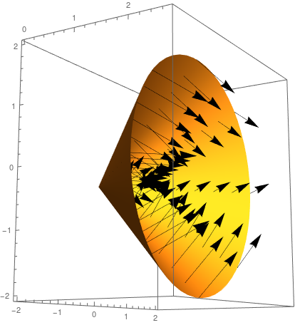
Example 1

The cone $x = \sqrt{y^2+z^2}, \, 0\le x\le 2,$ oriented in the direction of the positive $x$-axis. The boundary curve $\partial S$ is the circle $y^2+z^2 = 4,\, x=2$ oriented counter-clockwise when viewed from the positive $x$-axis.

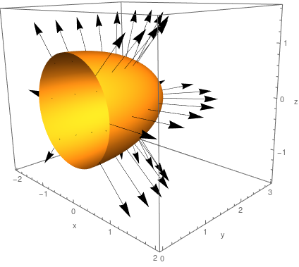
Example 2

The half of the ellipsoid $4x^2 + y^2 + 4z^2 = 4$ that lies to the right of the $xz$-plane, oriented in the direction of the positive $y$-axis. The boundary curve $\partial S$ is the circle $x^2+z^2=1,\, y=0$ oriented clockwise in the $xz$-plane.

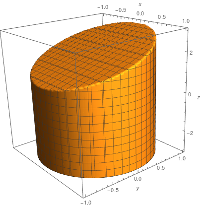
Example 3

The graph below is the region between the plane $z = y+2$ and the cylinder $x^2+y^2 = 1$. The surface $S$ is the plane $z=y+2$ within the cylinder. The curve $C = \partial S$ is an ellipse.

Example 4

Graphs of the cylinder $x^2 + y^2 = 1$ and the hyperbolic paraboloid $z = x^2 - y^2$. The surface $S$ is the part of the hyperbolic paraboloid within the cylinder.

xxxxxxxxxx

from sage.plot.plot3d.plot3d import axes;

from sage.plot.plot3d.parametric_surface import ParametricSurface;

​

x,y,u,v = var('x','y','u','v');

H = plot3d(x^2-y^2, (x,-1,1), (y,-1,1), frame = False, adaptive = True, color = ['blue', 'orange']);

C = parametric_plot3d((cos(u), sin(u), v), (u,0, 2*pi), (v,-2,2), frame = False, opacity=.8);

T = axes(2, .5);

show(H + C + T);

Curve of intersection of the above surfaces, given by the vector equation $\mathbf{r}(t) = \left<\cos u, \sin u, \cos 2t \right>$. This is the boundary curve $\partial S$.

xxxxxxxxxx

from sage.plot.plot3d.plot3d import axes;

u = var('u');

J = parametric_plot3d((cos(u), sin(u), cos(2*u)), (0,2*pi), frame=False, color='red');

T = axes(2, .5);

show(J+T);