Lecture 10: Section 2.2 Equilibrium Solution and Stability

(I) Equilibrium Solution

In previous sections we have often used explicit solutions of differential equations to answer specific numerical questions. But even when a given differential equation is difficult or impossible to solve, it is often possible to extract qualitative information about general properties of its solution. For example, as time $t$ approaches infinity, $x(t)$ grows without bound or approaches a finite limit.

Consider an autonomous first-order differential equation in which the independent variable $t$ does not appear explicitly:

\frac{dx}{dt} = f(x)

The solutions of $f(x) = 0$ are called critical points. If $x = c$ is a critical point, then the constant-valued function $x(t) \equiv c$ is called an equilibrium solution.

(II) Stability of Critical Points

Example 1

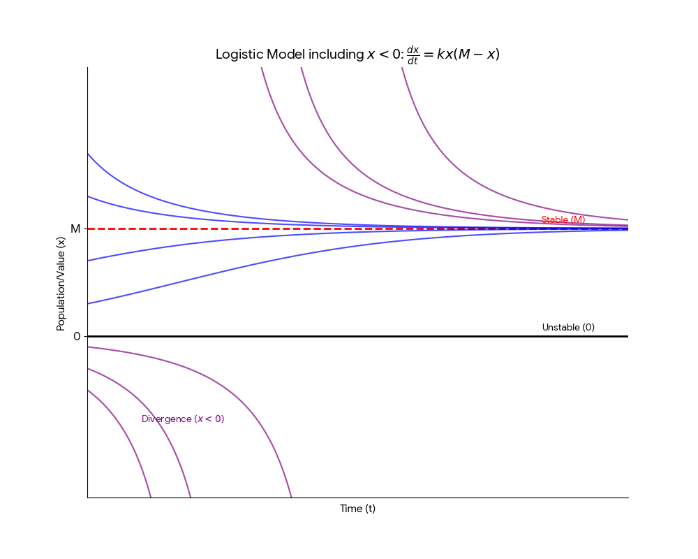
Consider the logistic differential equation: $$\frac{dx}{dt} = kx(M - x) \quad \text{with } x(0) = x_0$$

Critical Points: $f(x) = kx(M - x) = 0 \implies x = 0, M$. This yields two equilibrium solutions: $x \equiv 0$ and $x \equiv M$.

Behavior analysis:

If the initial population $x_0 > 0$, then $x(t)$ approaches $M$ as $t$ approaches infinity.
If $x_0 < 0$, the denominator is positive initially and then vanishes.

Phase Diagram Analysis:

When $0 < x < M$, then $x' > 0$.
When $x > M$, then $x' < 0$.
When $x < 0$, then $x' < 0$.

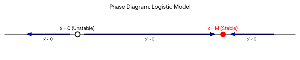
A horizontal phase diagram for the logistic equation. A red dot at M represents a stable equilibrium with arrows pointing toward it. An open circle at 0 represents an unstable equilibrium with arrows pointing away from it. — Phase Diagram of x' = kx(M - x)

Graphically, every solution either approaches $x \equiv M$ as $t$ increases or diverges away from $x \equiv 0$. Thus, $M$ is a stable critical point and $0$ is an unstable critical point.

Logistic model plot showing curves for x > M (falling to M), 0 < x < M (rising to M), and x < 0 (falling sharply away from 0 toward negative infinity). — Figure: Full Phase Analysis of x' = kx(M - x) including negative regions.

Example 2

Consider the explosion / extinction equation: $$\frac{dx}{dt} = kx(x - M)$$

Critical points: $kx(x - M) = 0 \implies x = 0, M$.

Phase diagram analysis:

If $x > M$, then $x' > 0$ (explosion).
If $0 < x < M$, then $x' < 0$ (extinction).
If $x < 0$, then $x' > 0$.

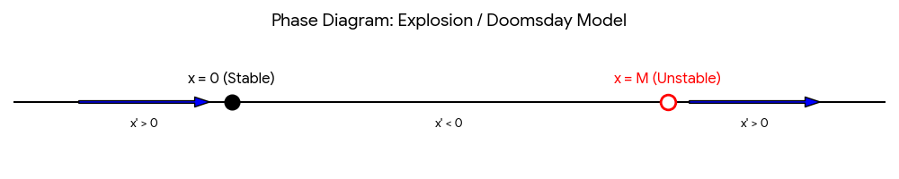
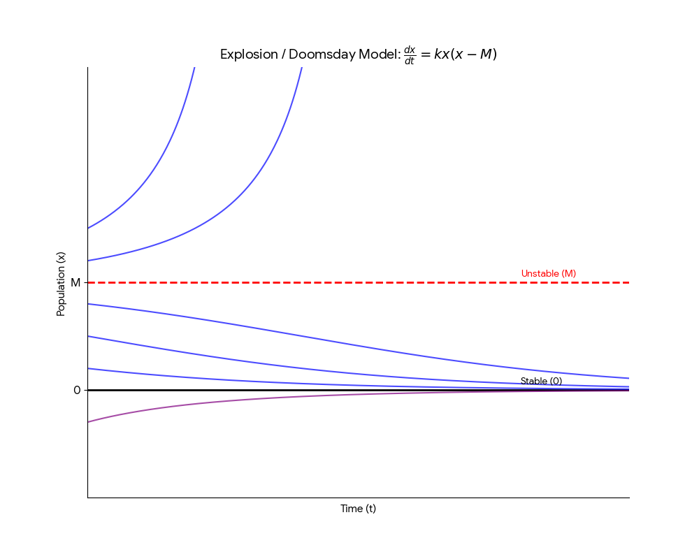
Phase diagram for the explosion model showing M as unstable and 0 as stable. — Phase Diagram for x' = kx(x - M)

Solution curves for the explosion model. Curves above M go to infinity, curves below M go to zero. — Solution Curves for x' = kx(x - M)

In this case, $0$ is a stable equilibrium and $M$ is an unstable equilibrium.

(III) Harvesting a Logistic Population

Consider the population of fish in a lake from which $h$ fish per year are removed by fishing:

\frac{dx}{dt} = kx(M - x) - h

Example 3: Harvesting a Logistic Population

Suppose that $k = 1, M = 4$ for a logistic population $x(t)$ of fish in a lake, measured in hundreds after $t$ years.

(a) Suppose harvesting level $h = 3$ (300 fish are harvested annually):

Find all the critical points and equilibrium solutions. Check the stability.

$$\frac{dx}{dt} = x(4 - x) - 3 = -x^2 + 4x - 3 = -(x - 1)(x - 3) = 0$$

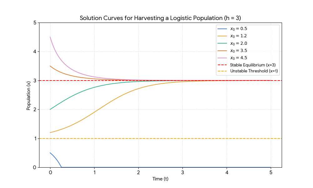
Critical points are $x = 1$ and $x = 3$. Stability check: $x = 3$ is a stable equilibrium limiting solution and $x = 1$ is an unstable threshold solution that separates different behavior.

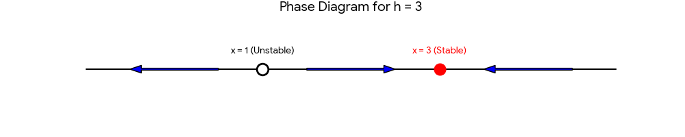
A phase line for the harvesting equation with h=3. The line has critical points at x=1 and x=3. Arrows point toward 3 from both sides (stable) and away from 1 (unstable).

Phase diagram for h = 3: Arrows point toward the stable equilibrium at 3 and away from the unstable threshold at 1.

The population approaches 300 if the initial population $x_0 > 1$. It becomes extinct because of harvesting if $x_0 < 1$.

Solution curves for h=3 showing stabilization at x=3 for x0>1 and extinction for x0<1. — Solution Curves for h = 3 (Stable at x=3, Unstable at x=1)

(b) Investigating the dependence of this picture upon the harvesting level $h$:

$$\frac{dx}{dt} = x(4 - x) - h \implies -x^2 + 4x - h = 0$$

Critical points are $c = \frac{1}{2}(4 \pm \sqrt{16 - 4h}) = 2 \pm \sqrt{4 - h}$.

Case 1 (harvesting level $h < 4$): There are two distinct equilibrium solutions $x(t) \equiv N$ and $x(t) \equiv H$ with $N > H$. This case is similar to Part (a).
Case 2 (harvesting level $h = 4$): $N = H = 2$. There is only one equilibrium solution $x(t) \equiv 2$, which is semistable.

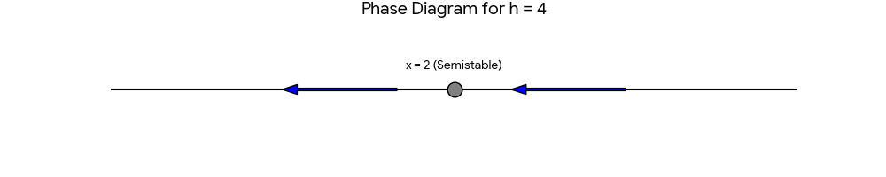
Phase diagram for h = 4: The equilibrium at x = 2 is semistable.

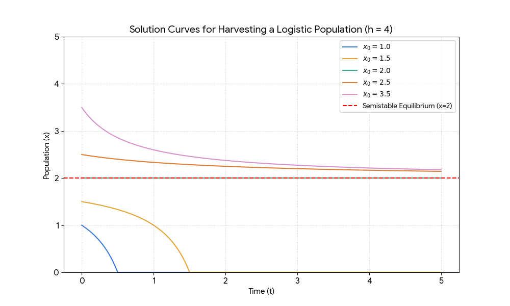
Solution Curves for h = 4
Case 3 (harvesting level $h > 4$): There is no real solution and no equilibrium solution. The population dies out as a result of excessive harvesting.

The value $h = 4$, for which the qualitative nature of the solutions changes as $h$ increases, is called a bifurcation point for the differential equation containing parameter $h$.

The bifurcation diagram consists of all points $(h, c)$ where $c$ is a critical point of the equation $x' = x(4 - x) - h$.

Since $c = 2 \pm \sqrt{4 - h}$, we have $(c - 2)^2 = 4 - h$.

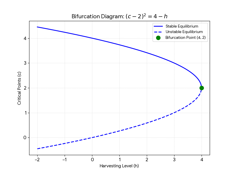
A bifurcation diagram showing harvesting level h on the horizontal axis and critical points c on the vertical axis. A parabola opens to the left with its vertex at the point (4, 2), representing the curve (c-2)^2 = 4-h.

Bifurcation diagram: The parabola separates regions of two, one (semistable), or no equilibrium solutions based on h.