Lecture 12: Sections 2.4 & 2.5 Numerical Approximation Methods

Introduction

In Chapter 1, we learned how to solve several specific types of first-order differential equations:

Separable
Linear (using the integrating factor $ e^{\int f(x) dx} $)
Homogeneous (using the substitution $ u = \frac{y}{x} $)
Bernoulli (using the substitution $ u = y^{1-n} $)
Exact (checking the criterion $ \frac{\partial M}{\partial y} = \frac{\partial N}{\partial x} $)

Consider the population model defined by the Initial Value Problem:

$$ \frac{dP}{dt} = f(t, P), \quad P(t_0) = P_0 $$

If the model is not one of these five types, how can we predict the population after 20 years? We use Numerical Methods.

Section 2.4 Numerical Approximation: Euler's Method

Consider an Initial Value Problem: $$\frac{dy}{dx} = f(x, y), \quad y(x_0) = y_0$$

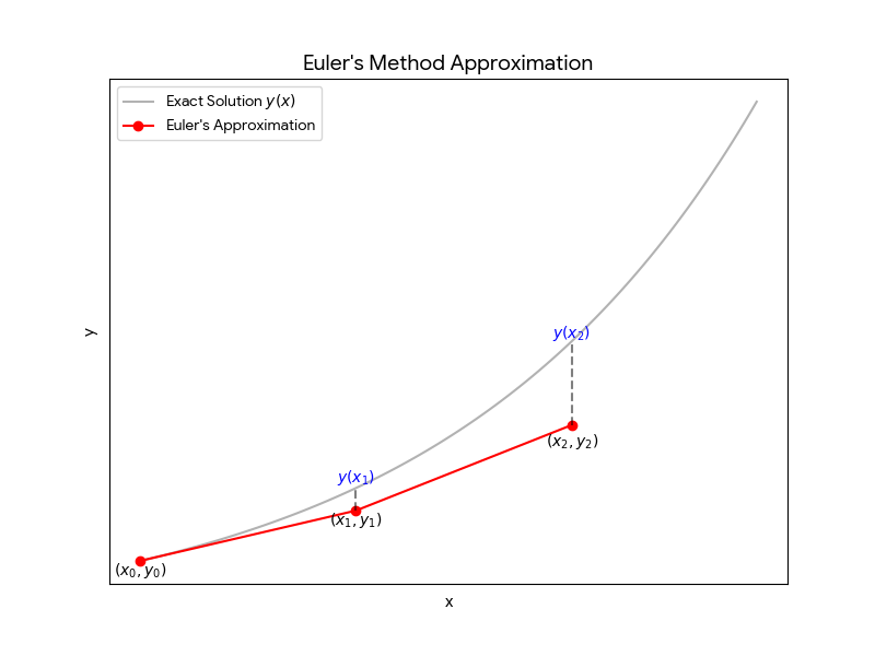
The slope of the tangent line to the solution curve at a point $ (x, y) $ is $ f(x, y) $. We would like to estimate the $ y $-value at some $ x $-value, say $ x_n $. Euler's Method is to use small tangent lines over a short distance to approximate the solution to the Initial Value Problem.

A graph showing a smooth exact solution curve y(x) starting at (x0, y0). A sequence of straight red line segments approximates the curve, moving from (x0, y0) to (x1, y1) and then to (x2, y2) based on the local slope at each approximation point.

Euler's Method: Tangent line segments approximating the solution curve.

The Algorithm and Formula

1. Choose a fixed horizontal step size $ h $ to use in making each step from one point to the next.

2. The equation of the tangent line at $ (x_0, y_0) $ is $ y - y_0 = m(x - x_0) $, where the slope $ m = \frac{dy}{dx}\big|_{(x_0, y_0)} = f(x_0, y_0) $.

3. To find the approximation for the first step ($ n = 1 $): $ y(x_1) \approx y_1 = y_0 + f(x_0, y_0)(x_1 - x_0) = y_0 + h \cdot f(x_0, y_0) $.

4. Use $ (x_1, y_1) $ as the initial point for the second step ($ n = 2 $) to find $ y_2 $, which approximates $ y(x_2) $: $ y(x_2) \approx y_2 = y_1 + f(x_1, y_1)(x_2 - x_1) = y_1 + h \cdot f(x_1, y_1) $.

In general, Euler's Method consists of applying the iterative formula:

y_{n+1} = y_n + h \cdot f(x_n, y_n), \quad (n \ge 0)

This formula calculates successive approximations $ y_1, y_2, \dots $ to the true values $ y(x_1), y(x_2), \dots $ of the exact solution $ y = y(x) $ at $ x_1, x_2, \dots $.

Remarks on Error

The error, $ |y(x_n) - y_n| $, decreases as the step size $ h $ is reduced.
The difference between the actual and approximate values typically increases as $ x $ gets farther from the starting point $ x_0 $.

Section 2.5 Improved Euler's Method (Predictor-Corrector Method)

Consider the Initial Value Problem: $ \frac{dy}{dx} = f(x, y), y(x_0) = y_0 $. Let $ h $ be the uniform step size where $ h = x_n - x_{n-1} $.

A coordinate graph showing the start point (xn, yn). Two slopes are visible: K1 (the slope at the start point) and K2 (the slope at the predicted point). The Improved Euler point (xn+1, yn+1) is calculated using the average of these two slopes.

Improved Euler's Method: Using average slope to calculate the corrected point.

The Two-Step Iteration

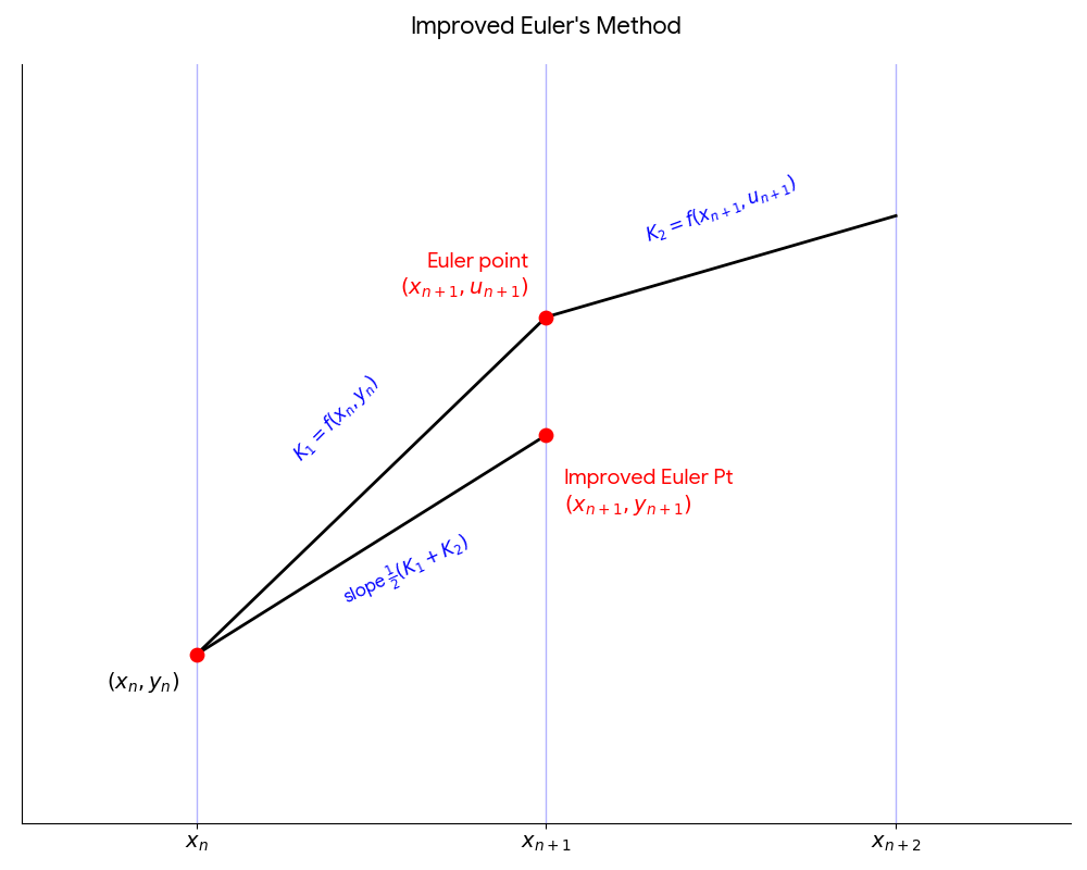
Use $ (x_n, y_n) $ to find the initial slope: $ k_1 = f(x_n, y_n) $.
Predictor Step: Use standard Euler's Method to find the intermediate predicted value: $ u_{n+1} = y_n + h \cdot f(x_n, y_n) $.
Use the predicted point $ (x_{n+1}, u_{n+1}) $ to find the second slope: $ k_2 = f(x_{n+1}, u_{n+1}) $.
Calculate the average of the two slopes: $ \frac{1}{2}(k_1 + k_2) $.
Corrector Step: Calculate the improved, corrected value: $ y_{n+1} = y_n + h \cdot \frac{1}{2}(k_1 + k_2) $.

Example 1

Consider the Initial Value Problem: $$\frac{dy}{dx} = x + y, \quad y(0) = 1$$

Estimate the solution of the Initial Value Problem at $ x = 0.2 $ using step size $ h = 0.1 $.

1. Euler's Method Analysis:

Starting with $ (x_0, y_0) = (0, 1) $ and $ f(x, y) = x + y $. Step count $ n = \frac{0.2 - 0}{0.1} = 2 $.

Step 1 ($ x_1 = 0.1 $): $ y_1 = y_0 + h \cdot f(x_0, y_0) = 1 + 0.1(0 + 1) = 1.1 $
Step 2 ($ x_2 = 0.2 $): $ y_2 = y_1 + h \cdot f(x_1, y_1) = 1.1 + 0.1(0.1 + 1.1) = \mathbf{1.22} $

2. Improved Euler's Method Analysis:

Step 1 ($ x_1 = 0.1 $): Starting at $ (x_0, y_0) = (0, 1) $.

$ k_1 = f(x_0, y_0) = 0 + 1 = 1 $
Predictor: $ u_1 = y_0 + h \cdot k_1 = 1 + 0.1 = 1.1 $
$ k_2 = f(x_1, u_1) = 0.1 + 1.1 = 1.2 $
Corrector: $ y_1 = y_0 + \frac{k_1 + k_2}{2} h = 1 + (1.1 \cdot 0.1) = 1.11 $

Step 2 ($ x_2 = 0.2 $): Starting at $ (x_1, y_1) = (0.1, 1.11) $.

$ k_1 = f(x_1, y_1) = 0.1 + 1.11 = 1.21 $
Predictor: $ u_2 = y_1 + h \cdot k_1 = 1.11 + 0.1(1.21) = 1.231 $
$ k_2 = f(x_2, u_2) = 0.2 + 1.231 = 1.431 $
Corrector: $ y_2 = y_1 + h \frac{k_1 + k_2}{2} = 1.11 + 0.1(1.3205) = \mathbf{1.24205} $

3. Comparison with Exact Solution:

The equation $ \frac{dy}{dx} - y = x $ is a first-order linear differential equation. Using the integrating factor $ e^{\int -1 dx} = e^{-x} $ and integration by parts:

$$ y(x) = -(x + 1) + 2e^x $$

The true value at $ x = 0.2 $ is $ y(0.2) = -1.2 + 2e^{0.2} \approx 1.2428 $.

Error using Euler's Method: $ |1.22 - 1.2428| = 0.0228 $
Error using Improved Euler's Method: $ |1.24205 - 1.2428| = 0.00075 $

The Improved Euler's Method is significantly more efficient. In fact, the error using Euler's is $ \le Ch $ while the error using Improved Euler's is $ \le Ch^2 $. Other methods, such as the Runge-Kutta Method, are $ \le Ch^4 $.

Extra Example: Computer-Aided Analysis

Use the Improved Euler method with a computer system to find the desired solution values. Start with step size $ h = 0.1 $, and then use successively smaller step sizes until successive approximate solution values at $ x = 2 $ agree rounded off to four decimal places.

Problem: $ y' = x^2 + y^2 - 1, \quad y(0) = 0 $. Find $ y(2) = ? $

For $ h = 0.1 $: Approximate solution $ y \approx 1.0109 $
For $ h = 0.05 $: Approximate solution $ y \approx 1.0062 $
For $ h = 0.01 $: Approximate solution $ y \approx 1.0045 $
For $ h = 0.005 $: Approximate solution $ y \approx 1.0045 $

Since the approximations agree at $ h = 0.01 $ and $ h = 0.005 $, we conclude $ y(2) \approx 1.0045 $.