Lecture 17: Section 3.4 Mechanical Vibrations

(I) Introduction: Mass-Spring-Dashpot System

We consider a mass-spring-dashpot system. A body of mass $ m $ is attached to one end of an ordinary spring that resists compression as well as stretching; the other end of the spring is attached to a fixed wall. We assume the body rests on a frictionless horizontal plane so that it can move only back and forth as the spring compresses and stretches.

System Parameters

$ x $: The distance of the body from its equilibrium position (the position when the spring is unstretched).
$ x > 0 $: The spring is stretched.
$ x < 0 $: The spring is compressed.
Restoring Force ($ F_S $): Defined by Hooke's Law as $ F_S = -kx $, where $ k > 0 $ is the spring constant.
Damping Force ($ F_R $): Provided by a dashpot (a device for shock/vibration damping). We assume the damping force is proportional to velocity: $ F_R = -cv = -c \frac{dx}{dt} $, where $ c > 0 $ is the damping constant.
External Force ($ F_E $): Represented as $ F(t) $.

The Equation of Motion

By Newton's Second Law, the total force $ F = ma = m x'' $. Summing the forces gives:

$$ m x'' + c x' + k x = F(t) $$

We categorize motion based on these constants:

$ c = 0 $: Undamped motion.
$ c > 0 $: Damped motion.
$ F(t) = 0 $: Free motion.
$ F(t) \neq 0 $: Forced motion.

(II) Free Undamped Motion

For free undamped motion ($ c = 0, F(t) = 0 $), the equation becomes $ m x'' + k x = 0 $. Dividing by $ m $ and letting $ \omega_0^2 = \frac{k}{m} $, we have:

x'' + \omega_0^2 x = 0

The general solution is $ x(t) = A \cos(\omega_0 t) + B \sin(\omega_0 t) $, where $ A $ and $ B $ are constants determined by initial conditions.

Detailed Step-by-Step: Converting to a Single Cosine Function

To better understand simple harmonic motion, we combine the sine and cosine terms into a single cosine function of the form: $$ x(t) = C \cos(\omega_0 t - \alpha) $$

Step 1: Define Amplitude $ C $. We utilize a right triangle where the horizontal side is $ A $ and the vertical side is $ B $. The hypotenuse $ C $ represents the amplitude: $$ C = \sqrt{A^2 + B^2} $$

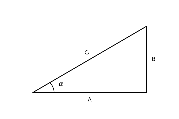
A right-angled triangle representing the relationship between coefficients A and B. The horizontal base is labeled A, the vertical side is labeled B, and the hypotenuse is labeled C. An angle alpha is located at the origin between sides A and C. The hypotenuse C represents the amplitude, calculated as the square root of A squared plus B squared. The angle alpha is the phase angle, where tangent of alpha equals B divided by A. — Figure: Reference Triangle for Amplitude (C) and Phase Angle (α)

Step 2: Define Phase Angle $ \alpha $. From the triangle, we see that: $$ \cos \alpha = \frac{A}{C}, \quad \sin \alpha = \frac{B}{C}, \quad \tan \alpha = \frac{B}{A} $$

Step 3: Quadrant Logic for $ \alpha $. When calculating $ \alpha = \arctan(B/A) $, you must check the signs of $ A $ and $ B $ to ensure $ \alpha $ is in the correct quadrant:

If $ A > 0, B > 0 $: $ \alpha = \arctan(B/A) $ (Quadrants I).
If $ A < 0 $: $ \alpha = \pi + \arctan(B/A) $ (Quadrants II or III).
If $ A >0, B<0 $: $ \alpha = 2\pi + \arctan(B/A) $ (Quadrants IV).

Step 4: The Derivation. We rewrite the original solution by factoring out $ C $: $$ x(t) = C \left( \frac{A}{C} \cos(\omega_0 t) + \frac{B}{C} \sin(\omega_0 t) \right) $$ Substituting $ \frac{A}{C} = \cos \alpha $ and $ \frac{B}{C} = \sin \alpha $: $$ x(t) = C \left( \cos \alpha \cos(\omega_0 t) + \sin \alpha \sin(\omega_0 t) \right) $$ Applying the trigonometric identity $ \cos(u - v) = \cos u \cos v + \sin u \sin v $, we arrive at: $$ x(t) = C \cos(\omega_0 t - \alpha) = C \cos\left(\omega_0 \left(t - \frac{\alpha}{\omega_0}\right)\right) $$

Motion Characteristics

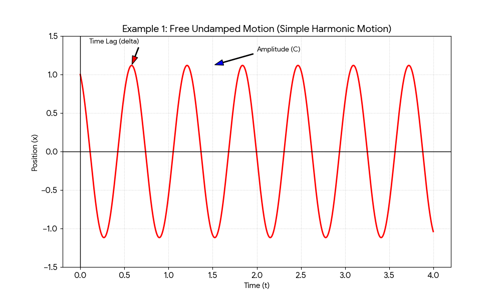
Amplitude ($ C $): The maximum displacement from equilibrium.
Circular Frequency ($ \omega_0 $): Measured in radians per second.
Period ($ T $): Time for one full oscillation, $ T = \frac{2\pi}{\omega_0} $.
Frequency ($ \nu $): Oscillations per second, $ \nu = \frac{1}{T} = \frac{\omega_0}{2\pi} $ (measured in Hertz).
Time Lag ($ \delta $): The time shift of the wave, $ \delta = \frac{\alpha}{\omega_0} $.

Example 1

A body with mass $ m = \frac{1}{2} $ kilogram is attached to a spring that is stretched 2 meters by a force of 100 Newtons. It is set in motion with initial position $ x_0 = 1 $ meter and initial velocity $ v_0 = -5 $ meters per second. Find the position function, amplitude, frequency, period, and time lag.

Step 1: Find the spring constant. $ k = \frac{100 \text{ N}}{2 \text{ m}} = 50 \text{ N/m} $.

Step 2: Set up the equation. $ \frac{1}{2}x'' + 50x = 0 \implies x'' + 100x = 0 $.
The characteristic equation is $ r^2 + 100 = 0 \implies r = \pm 10i $.
Thus, $ \omega_0 = 10 $ radians per second.

Step 3: Solve the Initial Value Problem.
$ x(t) = A \cos(10t) + B \sin(10t) $.
$ x(0) = A = 1 $.
$ x'(t) = -10A \sin(10t) + 10B \cos(10t) \implies x'(0) = 10B = -5 \implies B = -\frac{1}{2} $.
Position function: $ x(t) = \cos(10t) - \frac{1}{2} \sin(10t) $.

Step 4: Find characteristics.
Amplitude $ C = \sqrt{1^2 + (-\frac{1}{2})^2} = \frac{\sqrt{5}}{2} \approx 1.118 $.
Period $ T = \frac{2\pi}{10} = \frac{\pi}{5} \approx 0.6283 $ seconds.
Frequency $ \nu = \frac{5}{\pi} \approx 1.5915 $ Hertz.
Phase Angle: $ \tan \alpha = \frac{-1/2}{1} = -\frac{1}{2} $. Since $ \cos \alpha > 0 $ and $ \sin \alpha < 0 $, $ \alpha $ is in the 4th quadrant.
$ \alpha = 2\pi + \arctan(-1/2) \approx 5.8195 $ radians.
Time lag $ \delta = \frac{5.8195}{10} = 0.5820 $ seconds.

A coordinate plane showing a constant cosine wave for simple harmonic motion. The vertical axis represents displacement x and the horizontal axis represents time t. The wave oscillates between 1.118 and -1.118, which is the amplitude C calculated as square root of 5 divided by 2. The first peak is shifted from the origin by a time lag delta of approximately 0.582 seconds. The time between successive peaks represents the period T, which is pi divided by 5. — Figure: Simple Harmonic Motion for m=0.5kg and k=50N/m (Example 1)

(III) Free Damped Motion

The governing equation is $ m x'' + c x' + k x = 0 $. Letting $ 2p = \frac{c}{m} $ and $ \omega_0^2 = \frac{k}{m} $, we have:

x'' + 2p x' + \omega_0^2 x = 0

The characteristic roots are $ r_{1,2} = -p \pm \sqrt{p^2 - \omega_0^2} $. We define the critical damping constant as $ c_{cr} = \sqrt{4km} $.

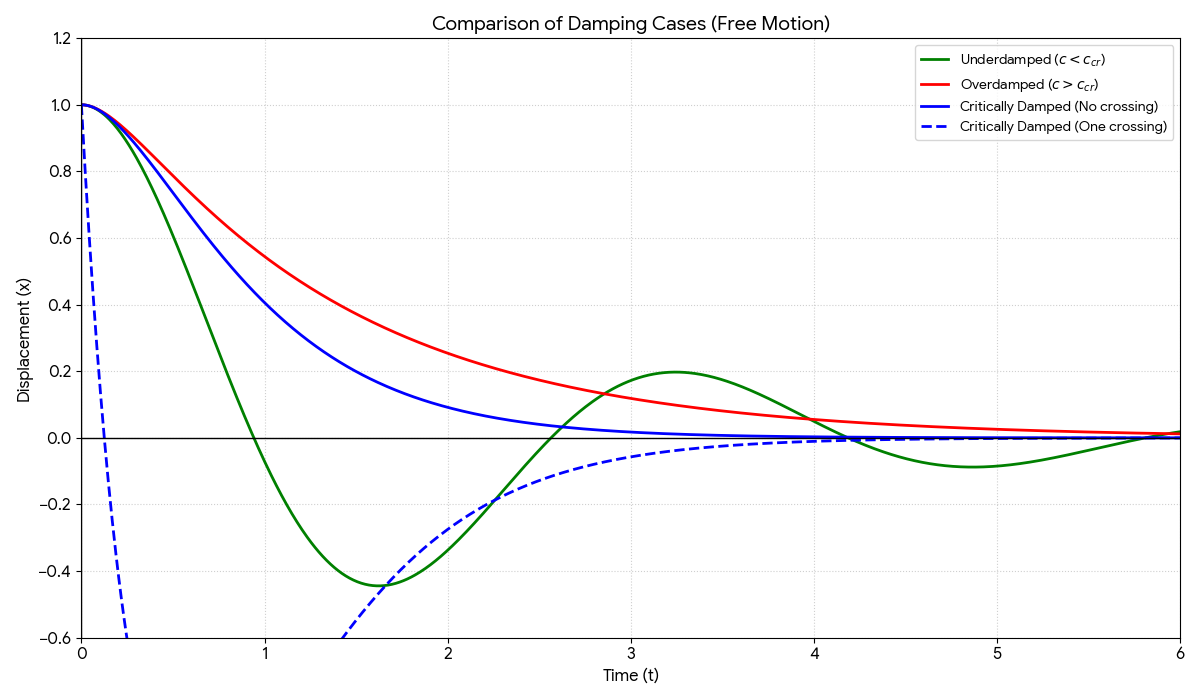
Case 1: Overdamped ($ c > c_{cr} $)

The roots are distinct, real, and negative. The solution is $ x(t) = C_1 e^{r_1 t} + C_2 e^{r_2 t} $. The body settles to equilibrium without any oscillations.

Case 2: Critically Damped ($ c = c_{cr} $)

The roots are repeated real roots $ r = -p $. The solution is $ x(t) = e^{-pt}(C_1 + C_2 t) $. The body passes through equilibrium at most once and does not oscillate.

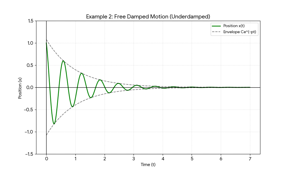
Case 3: Underdamped ($ c < c_{cr} $)

The roots are complex conjugates: $ -p \pm i \sqrt{\omega_0^2 - p^2} $. Let the pseudofrequency be $ \omega_1 = \sqrt{\omega_0^2 - p^2} $. The solution is:

x(t) = C e^{-pt} \cos(\omega_1 t - \alpha_1)

The time-varying amplitude is $ C e^{-pt} $, which exponentially damps the oscillations. The dashpot also decreases the frequency of motion ($ \omega_1 < \omega_0 $).

A line graph comparing four displacement-time curves for a mass-spring system. The green curve (Underdamped) oscillates multiple times while decaying. The red curve (Overdamped) returns to zero very slowly without crossing the axis. The solid blue curve (Critically Damped, No Crossing) returns to zero faster than the overdamped case. The dashed blue curve (Critically Damped, One Crossing) starts at a positive displacement, crosses the x-axis once to reach a negative peak, and then returns to equilibrium without crossing again. — Figure: Dynamics of Underdamped, Overdamped, and Critically Damped Systems

Example 2: Underdamped Motion Analysis

The mass and spring from Example 1 (mass $ m = 1/2 $ kilogram, spring constant $ k = 50 $ Newtons per meter) are now attached to a dashpot that provides 1 Newton of resistance for each meter per second of velocity. The system is set in motion with initial position $ x(0) = 1 $ meter and initial velocity $ x'(0) = -5 $ meters per second. Find the position function of the mass, its new frequency and pseudoperiod of motion, the new time lag, and the time of its first four passages through the equilibrium position $ x = 0 $.

Step 1: Set up the differential equation.
Using the parameters $ m = 1/2 $, $ c = 1 $, and $ k = 50 $, the equation of motion is: $$ \frac{1}{2}x'' + x' + 50x = 0 \implies x'' + 2x' + 100x = 0 $$ The characteristic equation is $ r^2 + 2r + 100 = 0 $. Using the quadratic formula: $$ r = \frac{-2 \pm \sqrt{4 - 400}}{2} = -1 \pm \sqrt{99}i $$ This is the underdamped case where the damping constant $ p = 1 $ and the pseudofrequency is $ \omega_1 = \sqrt{99} \approx 9.9499 $ radians per second.

Step 2: Find the general solution and solve for constants.
The general solution is $ x(t) = e^{-t}(A \cos\sqrt{99}t + B \sin\sqrt{99}t) $.
Applying the initial position $ x(0) = 1 $: $$ x(0) = e^0(A \cos(0) + B \sin(0)) = A = 1 $$ To find $ B $, we differentiate $ x(t) $: $$ x'(t) = -e^{-t}(A \cos\sqrt{99}t + B \sin\sqrt{99}t) + e^{-t}(-\sqrt{99}A \sin\sqrt{99}t + \sqrt{99}B \cos\sqrt{99}t) $$ Applying the initial velocity $ x'(0) = -5 $: $$ x'(0) = -A + \sqrt{99}B = -5 \implies -1 + \sqrt{99}B = -5 \implies \sqrt{99}B = -4 \implies B = -\frac{4}{\sqrt{99}} $$ The position function is: $ x(t) = e^{-t} \left( \cos\sqrt{99}t - \frac{4}{\sqrt{99}} \sin\sqrt{99}t \right) $.

Step 3: Convert to a single cosine function.
The amplitude constant is $ C_1 = \sqrt{A^2 + B^2} = \sqrt{1^2 + \left(-\frac{4}{\sqrt{99}}\right)^2} = \sqrt{\frac{115}{99}} \approx 1.077 $.
The phase angle $ \alpha_1 $ is determined by $ \tan \alpha_1 = \frac{B}{A} = -\frac{4}{\sqrt{99}} $. Since $ A > 0 $ and $ B < 0 $, $ \alpha_1 $ is in the fourth quadrant: $$ \alpha_1 = 2\pi - \arctan\left(\frac{4}{\sqrt{99}}\right) \approx 5.9009 \text{ radians} $$ The time-varying amplitude is $ \sqrt{\frac{115}{99}} e^{-t} $, and the simplified position function is: $$ x(t) \approx 1.077 e^{-t} \cos(\sqrt{99}t - 5.9009) $$

Step 4: Find motion characteristics.

Pseudoperiod ($ T_1 $): $ T_1 = \frac{2\pi}{\omega_1} = \frac{2\pi}{\sqrt{99}} \approx 0.6315 $ seconds.
Frequency ($ \nu_1 $): $ \nu_1 = \frac{1}{T_1} = \frac{\sqrt{99}}{2\pi} \approx 1.5836 $ Hertz.
Time Lag ($ \delta_1 $): $ \delta_1 = \frac{\alpha_1}{\omega_1} \approx \frac{5.9009}{9.9499} \approx 0.5931 $ seconds.

Step 5: Times of passage through equilibrium.
The mass passes through $ x = 0 $ when $ \cos(\omega_1 t - \alpha_1) = 0 $, which occurs at $ \omega_1 t - \alpha_1 = \dots, -\frac{3\pi}{2}, -\frac{\pi}{2}, \frac{\pi}{2}, \frac{3\pi}{2}, \dots $
Solving for $ t $: $ t = \delta_1 + \frac{(2n+1)\pi}{2\omega_1} $. The first four positive times are:

$ t_1 = \delta_1 - \frac{3\pi}{2\omega_1} \approx 0.1197 \text{ seconds} $
$ t_2 = \delta_1 - \frac{\pi}{2\omega_1} \approx 0.4354 \text{ seconds} $
$ t_3 = \delta_1 + \frac{\pi}{2\omega_1} \approx 0.7511 \text{ seconds} $
$ t_4 = \delta_1 + \frac{3\pi}{2\omega_1} \approx 1.0668 \text{ seconds} $

A graph showing underdamped motion where a sine wave starts at position x=1 and oscillates with decreasing amplitude. The wave is bounded by a dashed exponential envelope defined by the function sqrt(115/99) multiplied by e to the power of negative t. The peaks of the oscillations touch this envelope, showing the gradual decay of motion toward the equilibrium position x=0. The time between crossing points on the x-axis is slightly larger than in the undamped case, representing the pseudoperiod. — Figure: Underdamped Motion with Time-Varying Amplitude (Example 2)

Lecture 17 Section 3.4