(I) Introduction and Application
In this section, we transition from single differential equations to systems of differential equations. We define our variables as follows:
- Independent Variable: \( t \)
- Dependent Variables: \( x, y, z \) or \( x_1, x_2, x_3, \dots, x_n \)
We generally consider systems where the number of equations is equal to the number of dependent variables. For instance, a system with two equations and two dependent variables might look like:
\( f_2(t, x, y, x', y') = 0 \)
Application: Coupled Mass-Spring Systems
Consider a system of two masses and two springs. Let \( x(t) \) be the displacement of mass \( m_1 \) from its equilibrium position, and \( y(t) \) be the displacement of mass \( m_2 \) from its equilibrium position. An external force \( f(t) \) is applied to mass \( m_2 \).
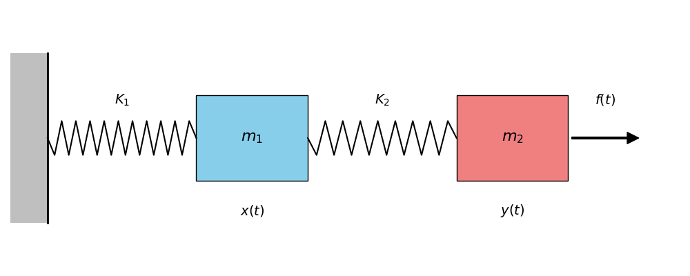
According to Newton's Second Law, the motion is described by the following system of second-order differential equations:
\( m_2 y'' = -k_2(y - x) + f(t) \)
(II) First-Order Systems
Any system of differential equations that can be solved for the highest-order derivatives of the dependent variables can be translated into an equivalent system of first-order differential equations. This transformation is the first step for many numerical techniques used with computers.
The Substitution Method
For an \( n^{th} \)-order differential equation \( x^{(n)} = f(t, x, x', \dots, x^{(n-1)}) \), we introduce \( n \) new variables:
This yields a system of \( n \) first-order equations:
\( x_2' = x_3 \)
\( \vdots \)
\( x_{n-1}' = x_n \)
\( x_n' = f(t, x_1, x_2, \dots, x_n) \)
Transform the following third-order differential equation into an equivalent system of first-order differential equations:
Solution: First, rewrite the equation solving for the highest derivative:
\( x^{(3)} = 5x - 2x' - 3x'' + \sin(2t) \)
Use the following substitutions:
\( x_1 = x, \quad x_2 = x', \quad x_3 = x'' \)
This yields the system:
\( x_1' = x_2 \)
\( x_2' = x_3 \)
\( x_3' = 5x_1 - 2x_2 - 3x_3 + \sin(2t) \)
Transform the following system of second-order equations into an equivalent system of first-order differential equations:
\( y'' = 2x - 2y + 40 \sin(3t) \)
Solution: Introduce four new variables:
\( x_1 = x, \quad x_2 = x', \quad y_1 = y, \quad y_2 = y' \)
This results in the first-order system:
\( x_1' = x_2 \)
\( x_2' = -3x_1 + y_1 \)
\( y_1' = y_2 \)
\( y_2' = 2x_1 - 2y_1 + 40 \sin(3t) \)
To transform a system of \( n \) first-order equations back into a single \( n^{th} \)-order equation, we use successive differentiation of the primary variable and substitute the other system equations to eliminate auxiliary variables.
Given the following system of three first-order differential equations, find the equivalent single third-order linear differential equation for the variable \( x_1 \):
(2) \( x_2' = x_3 \)
(3) \( x_3' = e^{2t} - 4x_1 + 3x_2 - 2x_3 \)
Derivation:
- From (1) and (2): \( x_1'' = x_2' = x_3 \)
- Differentiating again: \( x_1''' = x_3' \)
- Substitute \( x_2 = x_1' \), \( x_3 = x_1'' \) and \(x_3'= x_1''' \):
\( x_1''' = e^{2t} - 4x_1 + 3x_1' - 2x_1'' \)
Standard Form:
Result: This is the equivalent third-order linear differential equation.
(III) Simple 2-Dimensional Systems
Consider the linear second-order differential equation \( x'' + px' + qx = 0 \). By letting \( x = x \) and \( y = x' \), we can transform it into an equavalent two-dimensional system:
\( y' = -py - qx \)
Solve the two-dimensional system:
\( x' = -2y \)
\( y' = \frac{1}{2}x \)
Step 1: Convert to a second-order equation.
Differentiate the first equation: \( x'' = -2y' \).
Substitute the second equation into this: \( x'' = -2(\frac{1}{2}x) = -x \).
We have \( x'' + x = 0 \).
Step 2: Solve the second-order equation.
The characteristic equation is \( r^2 + 1 = 0 \implies r = \pm i \).
The general solution is \( x(t) = A \cos t + B \sin t \).
Step 3: Solve for \( y(t) \).
Since \( y = -\frac{1}{2}x' \), we calculate \( x'(t) = -A \sin t + B \cos t \).
Thus, \( y(t) = \frac{1}{2}A \sin t - \frac{1}{2}B \cos t \).
Step 4: Find the particular solution for \( x(0) = 2, y(0) = 0 \).
\( x(0) = A = 2 \).
\( y(0) = -\frac{1}{2}B = 0 \implies B = 0 \).
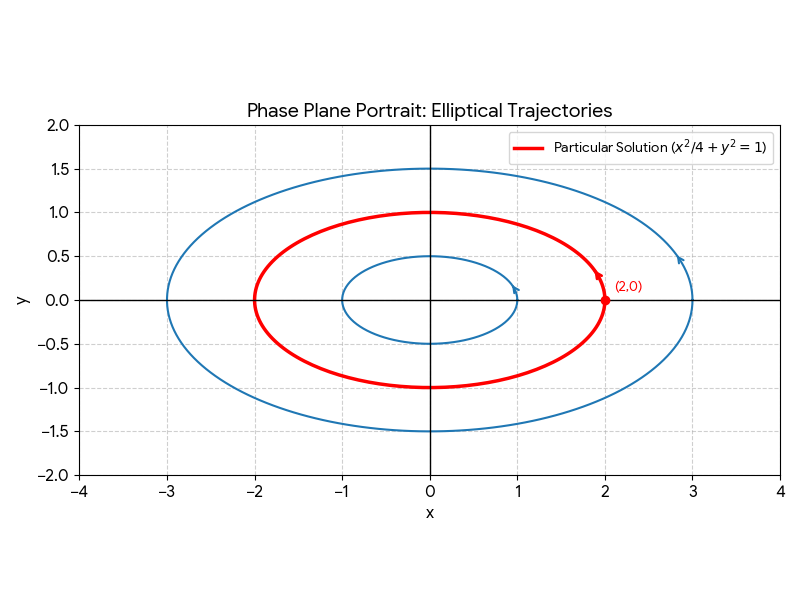
The solution is \( x(t) = 2 \cos t, y(t) = \sin t \).
Step 5: Identify the trajectory.
Using \( (\frac{x}{2})^2 + y^2 = \cos^2 t + \sin^2 t = 1 \).
This represents an ellipse in the \( xy \)-plane.
Definition: Phase Plane Portrait. A solution \( (x(t), y(t)) \) of a two-dimensional system may be regarded as a parametrization of a solution curve or trajectory in the \( xy \)-plane. The choice of initial conditions determines which trajectory a particular solution parametrizes. A collection of these trajectories is called a phase plane portrait.
(IV) Linear Systems
A linear first-order system with \( n \) equations has the following general form:
\( x_2' = p_{21}(t)x_1 + p_{22}(t)x_2 + \dots + p_{2n}(t)x_n + f_2(t) \)
\( \vdots \)
\( x_n' = p_{n1}(t)x_1 + p_{n2}(t)x_2 + \dots + p_{nn}(t)x_n + f_n(t) \)
The system is homogeneous if \( f_i(t) = 0 \) for all \( i \); otherwise, it is nonhomogeneous. A solution is an \( n \)-tuple of functions \( x_1(t), \dots, x_n(t) \) that satisfy each equation on an interval \( I \).
Theorem: Existence and Uniqueness for Linear Systems
Suppose that the coefficient functions \( p_{ij} \) and the functions \( f_i \) are continuous on an open interval \( I \) containing the point \( a \). Then the linear system with initial conditions \( x_i(a) = b_i \) for \( 1 \le i \le n \) has a unique solution on the interval \( I \).