Introduction: The Eigenvalue Method
We introduce a powerful alternative to the method of elimination to find the general solution of a homogeneous first-order linear system with constant coefficients of the form:
where \( \mathbf{A} \) is an \( n \times n \) matrix of constant coefficients. A general solution is a linear combination of \( n \) linearly independent solution vectors \( \vec{x}_1(t), \dots, \vec{x}_n(t) \).
Theorem 1: Eigenvalue Solution of \(\vec{x}' = \mathbf{A}\vec{x}\)
Let \(\lambda\) be the eigenvalue of the coefficient matrix \(\mathbf{A}\) of the first-order linear system \(\vec{x}' = \mathbf{A}\vec{x}\). If \(\vec{v}\) is an eigenvector associated with \(\lambda\), then:
is a nontrivial solution of the system.
Assuming a solution vector of the form \(\vec{x}(t) = \vec{v}e^{\lambda t}\) and substituting into the system yields:
Eigenvalues and Eigenvectors
A nontrivial solution \(\vec{x}(t) = \vec{v}e^{\lambda t}\) exists if and only if:
- Eigenvalue (\(\lambda\)): A scalar satisfying the characteristic equation: \[ \det(\mathbf{A} - \lambda \mathbf{I}) = 0 \]
- Eigenvector (\(\vec{v}\)): A non-zero column vector satisfying: \[ (\mathbf{A} - \lambda \mathbf{I})\vec{v} = \begin{bmatrix} 0 \\ \vdots \\ 0 \end{bmatrix} \]
Summary: The Eigenvalue Method
- Solve the characteristic equation \(\det(\mathbf{A} - \lambda \mathbf{I}) = 0\) for the eigenvalues \(\lambda_1, \dots, \lambda_n\).
- Find \(n\) linearly independent eigenvectors \(\vec{v}_1, \dots, \vec{v}_n\) associated with these eigenvalues.
- If \(n\) linearly independent eigenvectors exist, the general solution is:
\[ \vec{x}(t) = C_1\vec{v}_1e^{\lambda_1 t} + C_2\vec{v}_2e^{\lambda_2 t} + \dots + C_n\vec{v}_ne^{\lambda_n t} \]
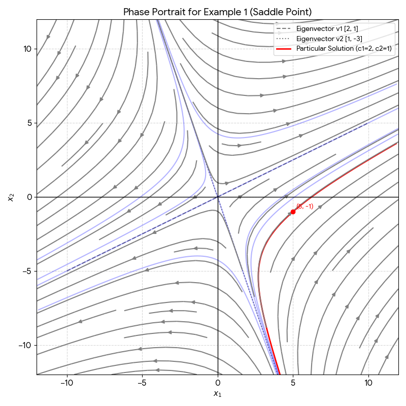
(I) Distinct Real Eigenvalues
Find the general solution and the particular solution satisfying \(\vec{x}(0) = \begin{bmatrix} 5 \\ -1 \end{bmatrix}\):
\( x_2' = 3x_1 - x_2 \)
Step 1: Eigenvalues. Solve \(\det(\mathbf{A} - \lambda \mathbf{I}) = 0\):
Step 2: Eigenvectors.
- For \(\lambda_1 = -2\): \( \mathbf{A} - (-2)\mathbf{I} = \begin{bmatrix} 6 & 2 \\ 3 & 1 \end{bmatrix} \sim \begin{bmatrix} 3 & 1 \\ 0 & 0 \end{bmatrix} \implies 3a + b = 0 \). Let \(a = 1 \implies \vec{v}_1 = \begin{bmatrix} 1 \\ -3 \end{bmatrix}\).
- For \(\lambda_2 = 5\): \( \mathbf{A} - 5\mathbf{I} = \begin{bmatrix} -1 & 2 \\ 3 & -6 \end{bmatrix} \sim \begin{bmatrix} 1 & -2 \\ 0 & 0 \end{bmatrix} \implies a - 2b = 0 \). Let \(b = 1 \implies \vec{v}_2 = \begin{bmatrix} 2 \\ 1 \end{bmatrix}\).
Step 3: Initial Value Problem. Using initial conditions yields \(C_1 = 1, C_2 = 2\):
Solve the system with matrix \(\mathbf{A} = \begin{bmatrix} 1 & 2 & 2 \\ 2 & 7 & 1 \\ 2 & 1 & 7 \end{bmatrix}\).
Step 1: Determinant calculation. Using row operation \(R_3 = -R_2 + R_3\):
This gives eigenvalues \(\lambda_1 = 0, \lambda_2 = 6, \lambda_3 = 9\).
Step 2: Eigenvectors using Row Reduction.
- For \(\lambda_1 = 0\): \( \begin{bmatrix} 1 & 2 & 2 \\ 2 & 7 & 1 \\ 2 & 1 & 7 \end{bmatrix} \xrightarrow{\substack{R_2-2R_1 \\ R_3-2R_1}} \begin{bmatrix} 1 & 2 & 2 \\ 0 & 3 & -3 \\ 0 & -3 & 3 \end{bmatrix} \sim \begin{bmatrix} 1 & 0 & 4 \\ 0 & 1 & -1 \\ 0 & 0 & 0 \end{bmatrix} \implies \begin{cases} a + 4c = 0 \\ b - c = 0 \end{cases} \implies \vec{v}_1 = \begin{bmatrix} -4 \\ 1 \\ 1 \end{bmatrix} \).
- For \(\lambda_2 = 6\): \( \begin{bmatrix} -5 & 2 & 2 \\ 2 & 1 & 1 \\ 2 & 1 & 1 \end{bmatrix} \sim \begin{bmatrix} 1 & 0 & 0 \\ 0 & 1 & 1 \\ 0 & 0 & 0 \end{bmatrix} \implies \begin{cases} a = 0 \\ b + c = 0 \end{cases} \implies \vec{v}_2 = \begin{bmatrix} 0 \\ 1 \\ -1 \end{bmatrix} \).
- For \(\lambda_3 = 9\): \( \begin{bmatrix} -8 & 2 & 2 \\ 2 & -2 & 1 \\ 2 & 1 & -2 \end{bmatrix} \sim \begin{bmatrix} 1 & 0 & -1/2 \\ 0 & 1 & -1 \\ 0 & 0 & 0 \end{bmatrix} \implies \begin{cases} a = c/2 \\ b = c \end{cases} \text{Let } c=2 \implies \vec{v}_3 = \begin{bmatrix} 1 \\ 2 \\ 2 \end{bmatrix} \).
General Solution: \( \vec{x}(t) = C_1 \begin{bmatrix} -4 \\ 1 \\ 1 \end{bmatrix} + C_2 \begin{bmatrix} 0 \\ 1 \\ -1 \end{bmatrix} e^{6t} + C_3 \begin{bmatrix} 1 \\ 2 \\ 2 \end{bmatrix} e^{9t} \).
(II) Compartmental Analysis
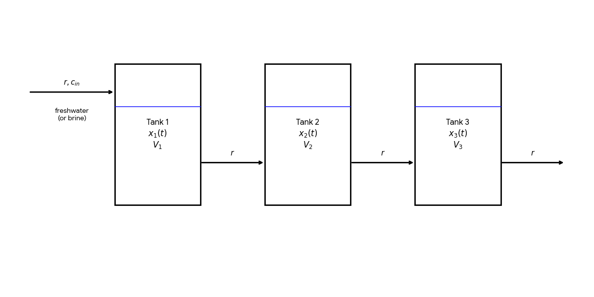
Complex systems are broken into compartments. For a cascading system of tanks with volume \(V_i\) and flow rate \(r\), the salt amount \(x_i\) is governed by:
\( \frac{dx_3}{dt} = k_2x_2 - k_3x_3 \)
\(\frac{dx_2}{dt} = k_1x_1 - k_2x_2\), \(\qquad\) where \(k_i = \frac{r}{V_i} \)
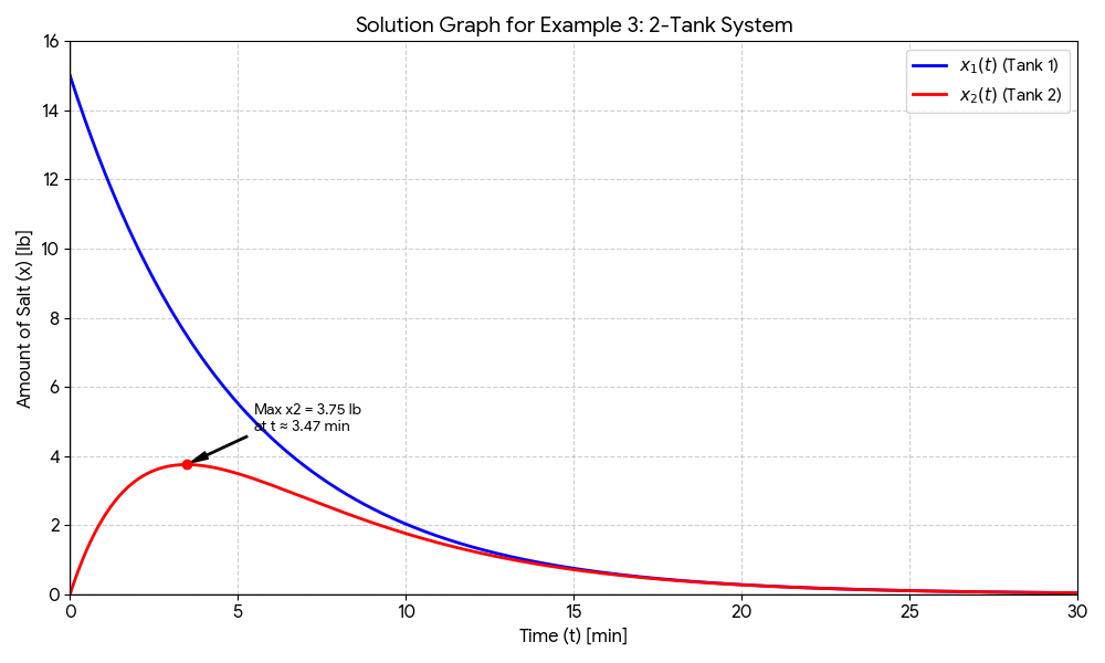
A two-tank system contains Tank 1 with volume \( V_1 = 50 \) gallons and Tank 2 with volume \( V_2 = 25 \) gallons. Initially, Tank 1 contains 15 pounds of salt and Tank 2 contains 0 pounds. Fresh water flows into Tank 1 at a rate of \( r = 10 \) gallons per minute, and the mixture cascades into Tank 2 and eventually out of the system at the same rate. Find the amount of salt in each tank at time \( t \) and the maximum amount of salt ever in Tank 2.
Step 1: System Setup.
The transfer coefficients are defined as \( k_i = \frac{r}{V_i} \):
\[ k_1 = \frac{10}{50} = \frac{1}{5}, \quad k_2 = \frac{10}{25} = \frac{2}{5} \]The system of differential equations is:
Step 2: Find Eigenvalues and Eigenvectors.
The characteristic equation is \( \det(\mathbf{A} - \lambda \mathbf{I}) = \left(-\frac{1}{5} - \lambda\right)\left(-\frac{2}{5} - \lambda\right) = 0 \), which gives eigenvalues \( \lambda_1 = -\frac{1}{5} \) and \( \lambda_2 = -\frac{2}{5} \).
- For \( \lambda_1 = -\frac{1}{5} \): \( \begin{bmatrix} 0 & 0 \\ \frac{1}{5} & -\frac{1}{5} \end{bmatrix} \begin{bmatrix} a \\ b \end{bmatrix} = \begin{bmatrix} 0 \\ 0 \end{bmatrix} \implies a = b \). Let \( a = 1 \implies \vec{v}_1 = \begin{bmatrix} 1 \\ 1 \end{bmatrix} \).
- For \( \lambda_2 = -\frac{2}{5} \): \( \begin{bmatrix} \frac{1}{5} & 0 \\ \frac{1}{5} & 0 \end{bmatrix} \begin{bmatrix} a \\ b \end{bmatrix} = \begin{bmatrix} 0 \\ 0 \end{bmatrix} \implies a = 0 \). Let \( b = 1 \implies \vec{v}_2 = \begin{bmatrix} 0 \\ 1 \end{bmatrix} \).
Step 3: General Solution.
Step 4: Solve for Constants (Particular Solution).
Apply the initial conditions \( x_1(0) = 15 \) and \( x_2(0) = 0 \):
\[ \vec{x}(0) = C_1 \begin{bmatrix} 1 \\ 1 \end{bmatrix} + C_2 \begin{bmatrix} 0 \\ 1 \end{bmatrix} = \begin{bmatrix} 15 \\ 0 \end{bmatrix} \implies \begin{cases} C_1 = 15 \\ C_1 + C_2 = 0 \implies C_2 = -15 \end{cases} \]The particular solution is:
Step 5: Find the Maximum Salt in Tank 2.
Set the derivative of \( x_2(t) \) to zero to find the critical point:
\[ x_2'(t) = -3e^{-t/5} + 6e^{-2t/5} = 0 \] \[ -3e^{-t/5}(1 - 2e^{-t/5}) = 0 \implies e^{-t/5} = \frac{1}{2} \] \[ t = 5 \ln 2 \approx 3.47 \text{ minutes} \]Substituting \( e^{-t/5} = \frac{1}{2} \) and \( e^{-2t/5} = \frac{1}{4} \) into the formula for \( x_2(t) \):
\[ x_2(5 \ln 2) = 15\left(\frac{1}{2}\right) - 15\left(\frac{1}{4}\right) = 7.5 - 3.75 = 3.75 \text{ pounds} \]Result: The maximum amount of salt ever in Tank 2 is 3.75 pounds.
(III) Distinct Complex Eigenvalues
Suppose a matrix \(\mathbf{A}\) has real entries. If \(\lambda = p + qi\) and \(\overline{\lambda} = p - qi\) are a conjugate pair of eigenvalues, let \(\vec{v}\) be an eigenvector associated with \(\lambda\). Then \(\overline{\vec{v}}\) is an eigenvector associated with \(\overline{\lambda}\). Both \(\vec{v}e^{\lambda t} \) and \(\overline{\vec{v}}e^{\overline{\lambda}t}\) are complex-valued solutions. We would like to derive two linearly independent real-value solutions from them.
Derivation of Real solutions
Let \(\vec{v} = \vec{a} + \vec{b}i\) and \(\lambda = p + qi\). The complex-valued solution \(\vec{v}e^{\lambda t}\) is expanded using Euler's formula:
\( \vec{v}e^{\lambda t} = (\vec{a} + \vec{b}i) e^{(p + qi)t} = e^{pt}(\vec{a} + \vec{b}i)(\cos(qt) + i \sin(qt)) \)Multiplying these terms yields:
\( \vec{v}e^{\lambda t} = e^{pt} \left[ (\vec{a} \cos(qt) - \vec{b} \sin(qt)) + i (\vec{b} \cos(qt) + \vec{a} \sin(qt)) \right] \)The two linearly independent real-valued solutions are the real and imaginary parts:
\( \vec{x}_1(t) = \text{Re}(\vec{v}e^{\lambda t}) = e^{pt}(\vec{a} \cos(qt) - \vec{b} \sin(qt)) \) \( \vec{x}_2(t) = \text{Im}(\vec{v}e^{\lambda t}) = e^{pt}(\vec{b} \cos(qt) + \vec{a} \sin(qt)) \)A real general solution is then written as
Solve: \(x_1' = 4x_1 - 3x_2\) and \(x_2' = 3x_1 + 4x_2\).
Step 1: Eigenvalues. \((\lambda - 4)^2 + 9 = 0 \implies \lambda = 4 \pm 3i\).
Step 2: Eigenvector calculation. For \(\lambda = 4 + 3i\):
\( \begin{bmatrix} -3i & -3 \\ 3 & -3i \end{bmatrix} \begin{bmatrix} a \\ b \end{bmatrix} = \begin{bmatrix} 0 \\ 0 \end{bmatrix} \implies -3ia - 3b = 0 \implies b = -ia \).
Let \(a = 1 \implies \vec{v} = \begin{bmatrix} 1 \\ -i \end{bmatrix} = \begin{bmatrix} 1 \\ 0 \end{bmatrix} + i\begin{bmatrix} 0 \\ -1 \end{bmatrix}\).
Step 3: Solution Derivation. Plugging into \(\vec{v}e^{\lambda t}\):
\(\vec{v}e^{\lambda t} = \begin{bmatrix} 1 \\ -i \end{bmatrix} e^{(4+3i)t} = e^{4t} \begin{bmatrix} 1 \\ -i \end{bmatrix} (\cos 3t + i \sin 3t) \) \(= e^{4t} \begin{bmatrix} \cos 3t + i \sin 3t \\ -i \cos 3t + \sin 3t \end{bmatrix} = e^{4t} \begin{bmatrix} \cos 3t \\ \sin 3t \end{bmatrix} + i e^{4t} \begin{bmatrix} \sin 3t \\ -\cos 3t \end{bmatrix} \)Final General Solution:
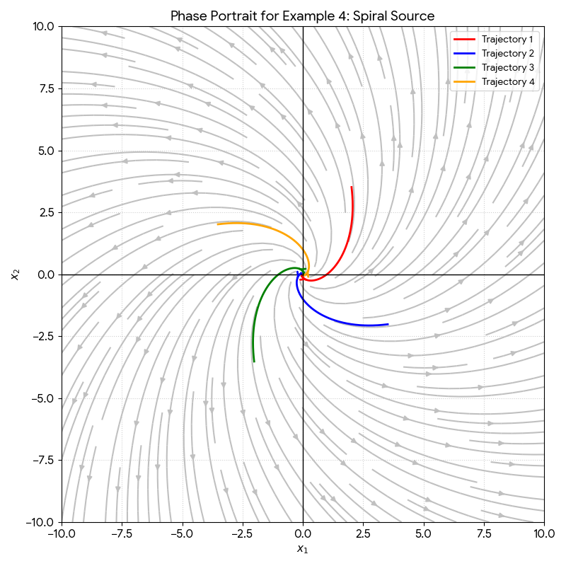
The origin is a spiral source because the real part of the eigenvalue (\( 4 \)) is positive. If it were negative, the origin would be a spiral sink.