(I) Introduction and Complete Eigenvalues
Previously, we saw that if an \( n \times n \) coefficient matrix \( \mathbf{A} \) has \( n \) distinct eigenvalues \( \lambda_1, \dots, \lambda_n \), the general solution is:
We now consider the case when the characteristic equation \( \det(\mathbf{A} - \lambda \mathbf{I}) = 0 \) has at least one repeated root.
Complete Eigenvalues
An eigenvalue \( \lambda \) of multiplicity \( k \) is complete if it has \( k \) linearly independent associated eigenvectors.
If all eigenvalues of \( \mathbf{A} \) are complete, there exists a complete set of \( n \) linearly independent eigenvectors \( \vec{v}_1, \dots, \vec{v}_n \) corresponding to \( \lambda_1 , \dots, \lambda_n \) (each repeated with its multiplicity), and the general solution remains:
Find the general solution of:
Step 1: Characteristic Equation.
Eigenvalues: \( \lambda_1 = 5 \) (multiplicity 1) and \( \lambda_2 = 3 \) (multiplicity 2).
Step 2: Find Eigenvectors.
- For \( \lambda_1 = 5 \): \( (\mathbf{A} - 5\mathbf{I})\vec{v} = \vec{0} \implies \begin{bmatrix} 4 & 4 & 0 \\ -6 & -6 & 0 \\ 6 & 4 & -2 \end{bmatrix} \sim \begin{bmatrix} 1 & 0 & -1 \\ 0 & 1 & 1 \\ 0 & 0 & 0 \end{bmatrix} \implies \vec{v}_1 = \begin{bmatrix} 1 \\ -1 \\ 1 \end{bmatrix} \).
- For \( \lambda_2 = 3 \): \( (\mathbf{A} - 3\mathbf{I})\vec{v} = \vec{0} \implies \begin{bmatrix} 6 & 4 & 0 \\ -6 & -4 & 0 \\ 6 & 4 & 0 \end{bmatrix} \sim \begin{bmatrix} 3 & 2 & 0 \\ 0 & 0 & 0 \\ 0 & 0 & 0 \end{bmatrix} \implies 3a + 2b = 0 \).
This gives two linearly independent eigenvectors for \( \lambda = 3 \):
General Solution:
(II) Defective Eigenvalues
An eigenvalue of multiplicity \( k \) is defective if it has fewer than \( k \) linearly independent associated eigenvectors. The difference \( d = k - p \) (where \( p \) is the number of independent eigenvectors) is called the defect.
Defective Eigenvalue of Multiplicity 2
If there is only one linearly independent eigenvector \( \vec{v}_1 \), we cannot use the standard form. Instead, we find a second solution of the form:
Substituting into \( \vec{X}' = \mathbf{A}\vec{X} \) leads to the following relations:
- \( (\mathbf{A} - \lambda \mathbf{I})\vec{v}_1 = \vec{0} \) (\( \vec{v}_1 \) is an eigenvector)
- \( (\mathbf{A} - \lambda \mathbf{I})\vec{v}_2 = \vec{v}_1 \) (\( \vec{v}_2 \) is a generalized eigenvector)
Algorithm for Multiplicity 2
- Find a non-zero solution \( \vec{v}_2 \) to \( (\mathbf{A} - \lambda \mathbf{I})^2 \vec{v}_2 = \vec{0} \) such that \( (\mathbf{A} - \lambda \mathbf{I})\vec{v}_2 = \vec{v}_1 \neq \vec{0} \).
- Construct the general solution: \[ \vec{X}(t) = C_1 \vec{v}_1 e^{\lambda t} + C_2 (\vec{v}_1 t + \vec{v}_2)e^{\lambda t} \]
Find the general solution of: \( \vec{X}' = \begin{bmatrix} 1 & -3 \\ 3 & 7 \end{bmatrix} \vec{X} \).
Step 1: Eigenvalues.
\[ \det(\mathbf{A} - \lambda \mathbf{I}) = \lambda^2 - 8\lambda + 16 = (\lambda - 4)^2 = 0 \implies \lambda = 4 \text{ (multiplicity 2)} \]Step 2: Find Generalized Eigenvectors.
\[ \mathbf{A} - 4\mathbf{I} = \begin{bmatrix} -3 & -3 \\ 3 & 3 \end{bmatrix}, \quad (\mathbf{A} - 4\mathbf{I})^2 = \begin{bmatrix} 0 & 0 \\ 0 & 0 \end{bmatrix} \]Pick \( \vec{v}_2 = \begin{bmatrix} 1 \\ 0 \end{bmatrix} \). Then \( \vec{v}_1 = (\mathbf{A} - 4\mathbf{I})\vec{v}_2 = \begin{bmatrix} -3 \\ 3 \end{bmatrix} \neq \vec{0} \).
General Solution:
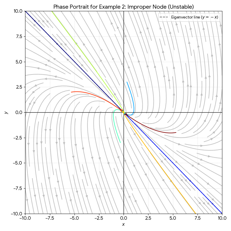
The origin is called an improper nodal source. Trajectories become tangent to the line \( x_1 = -x_2 \) as \( t \to \infty \).
(III) Generalized Eigenvectors
A rank \( r \) generalized eigenvector associated with eigenvalue \( \lambda \) is a vector \( \vec{u} \) such that:
- Rank 1 (\( r=1 \)): Standard eigenvector.
- Rank 2 (\( r=2 \)): The vector \( \vec{v}_2 \) in the multiplicity 2 algorithm.
Algorithm for Length 3 Chain
- Find a rank 3 generalized eigenvector \( \vec{v}_3 \) such that \( (\mathbf{A} - \lambda \mathbf{I})^3 \vec{v}_3 = \vec{0} \).
- Define \( \vec{v}_2 = (\mathbf{A} - \lambda \mathbf{I})\vec{v}_3 \).
- Define \( \vec{v}_1 = (\mathbf{A} - \lambda \mathbf{I})\vec{v}_2 \).
- The solutions are:
\( \vec{X}_1(t) = \vec{v}_1 e^{\lambda t} \)
\( \vec{X}_2(t) = (\vec{v}_1 t + \vec{v}_2) e^{\lambda t} \)
\( \vec{X}_3(t) = \left( \frac{1}{2}\vec{v}_1 t^2 + \vec{v}_2 t + \vec{v}_3 \right) e^{\lambda t} \)