Introduction: Equilibrium and Stability
Let \(\mathbf{A}\) be a \(2 \times 2\) matrix and \(\det \mathbf{A} \neq 0\). Consider the homogeneous linear system:
\(\vec{x} = \vec{0}\) is the equilibrium solution. Proof: \(\vec{x}' = \vec{0} \implies \mathbf{A}\vec{x} = \vec{0} \implies \vec{x} = \mathbf{A}^{-1}\vec{0} = \vec{0}\). We use the phase plane (\(x_1\)-\(x_2\) plane) to determine the stability of the equilibrium solution (the origin). Let \(\lambda_1\) and \(\lambda_2\) be the eigenvalues of \(\mathbf{A}\).
(I) \(\lambda_{1} \neq \lambda_{2}\): Distinct Real Eigenvalues
The general solution is \(\vec{x}(t) = C_1\vec{v}_1e^{\lambda_1 t} + C_2\vec{v}_2e^{\lambda_2 t}\).
Case 1: \(\lambda_1 < 0 < \lambda_2\) (Saddle Point)
From Section 5.2 Example 1, where \(\lambda_1 = -2\) and \(\lambda_2 = 5\):
Analysis:
- If \(C_2 = 0 \implies x_2 = -3x_1\). This is line \(\ell_1\) passing through \(\vec{v}_1\) and the origin.
- If \(C_1 = 0 \implies x_1 = 2x_2\). This is line \(\ell_2\) passing through \(\vec{v}_2\) and the origin.
- If \(C_1 \neq 0, C_2 \neq 0\): As \(t \to \infty\), solution curves extend asymptotically toward \(\ell_2\). As \(t \to -\infty\), solution curves extend asymptotically toward \(\ell_1\).
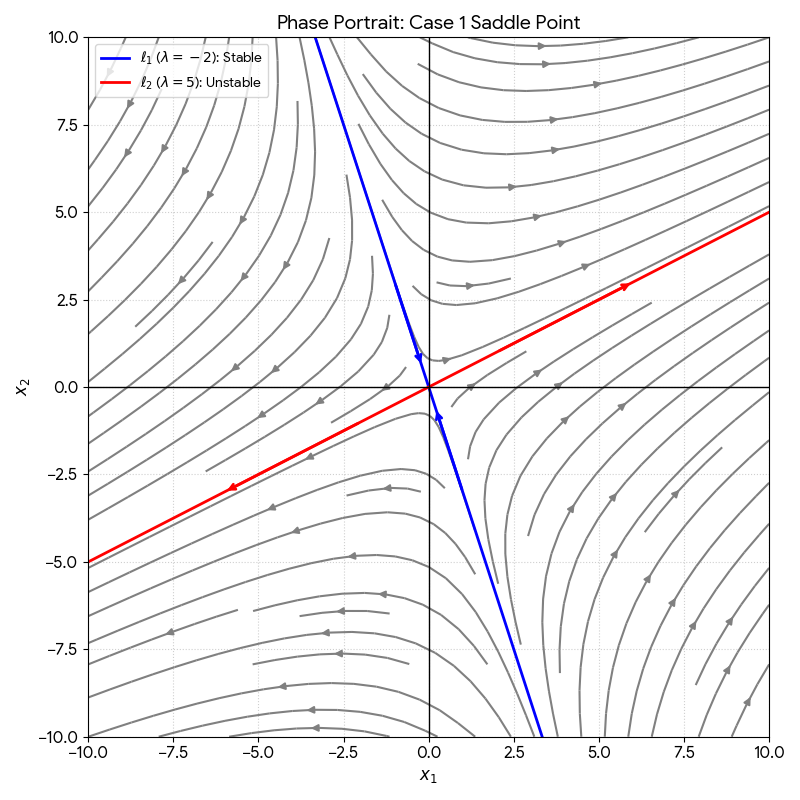
The origin is called a saddle point. It is unstable. Note that \(\vec{v}_1\) (with \(\lambda_1 < 0\)) points to the origin, while \(\vec{v}_2\) (with \(\lambda_2 > 0\)) points outward.
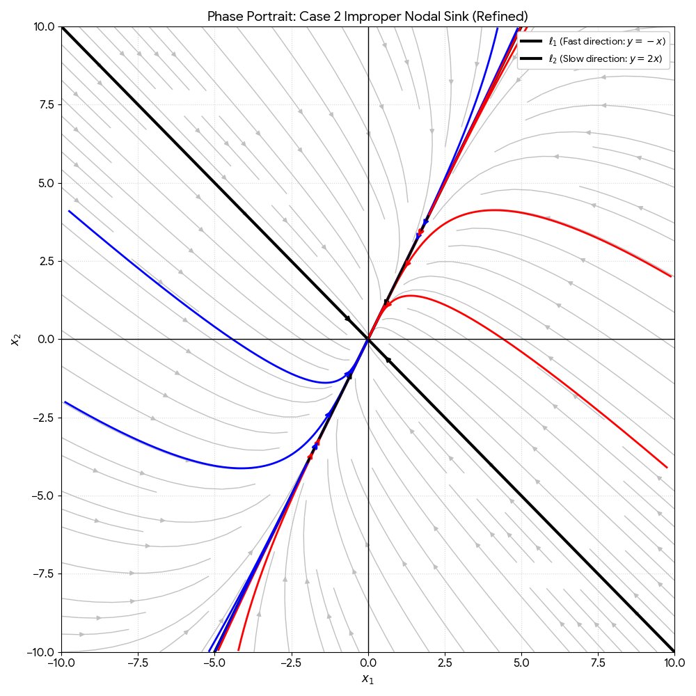
Case 2: \(\lambda_1 < \lambda_2 < 0\) (Improper Nodal Sink)
Consider \(\vec{x}' = \begin{bmatrix} -3 & 1 \\ 2 & -2 \end{bmatrix} \vec{x}\).
Step 1: Eigenvalues. \(\det(\mathbf{A} - \lambda \mathbf{I}) = \lambda^2 + 5\lambda + 4 = (\lambda + 1)(\lambda + 4) = 0 \implies \lambda_1 = -4, \lambda_2 = -1\).
Step 2: Eigenvectors. For \(\lambda_1 = -4, \vec{v}_1 = \begin{bmatrix} 1 \\ -1 \end{bmatrix}\). For \(\lambda_2 = -1, \vec{v}_2 = \begin{bmatrix} 1 \\ 2 \end{bmatrix}\).
Step 3: Solution Analysis. \(\vec{x}(t) = C_1 \begin{bmatrix} 1 \\ -1 \end{bmatrix} e^{-4t} + C_2 \begin{bmatrix} 1 \\ 2 \end{bmatrix} e^{-t}\).
As \(t \to \infty\), all solutions approach the origin. Because \(e^{-4t}\) decays faster than \(e^{-t}\), trajectories become tangent to line \(\ell_2\) passing through \(\vec{v}_2\) as \(t \to \infty\).
Case 3: \(0 < \lambda_2 < \lambda_1\) (Improper Nodal Source)
Similar to Case 2, but trajectories move away from the origin as \(t\) increases (the direction of motion along each solution curve is reversed). The origin is an improper nodal source and is unstable.
(II) \(\lambda_1 = \lambda_2 = \lambda\): Repeated Real Eigenvalues
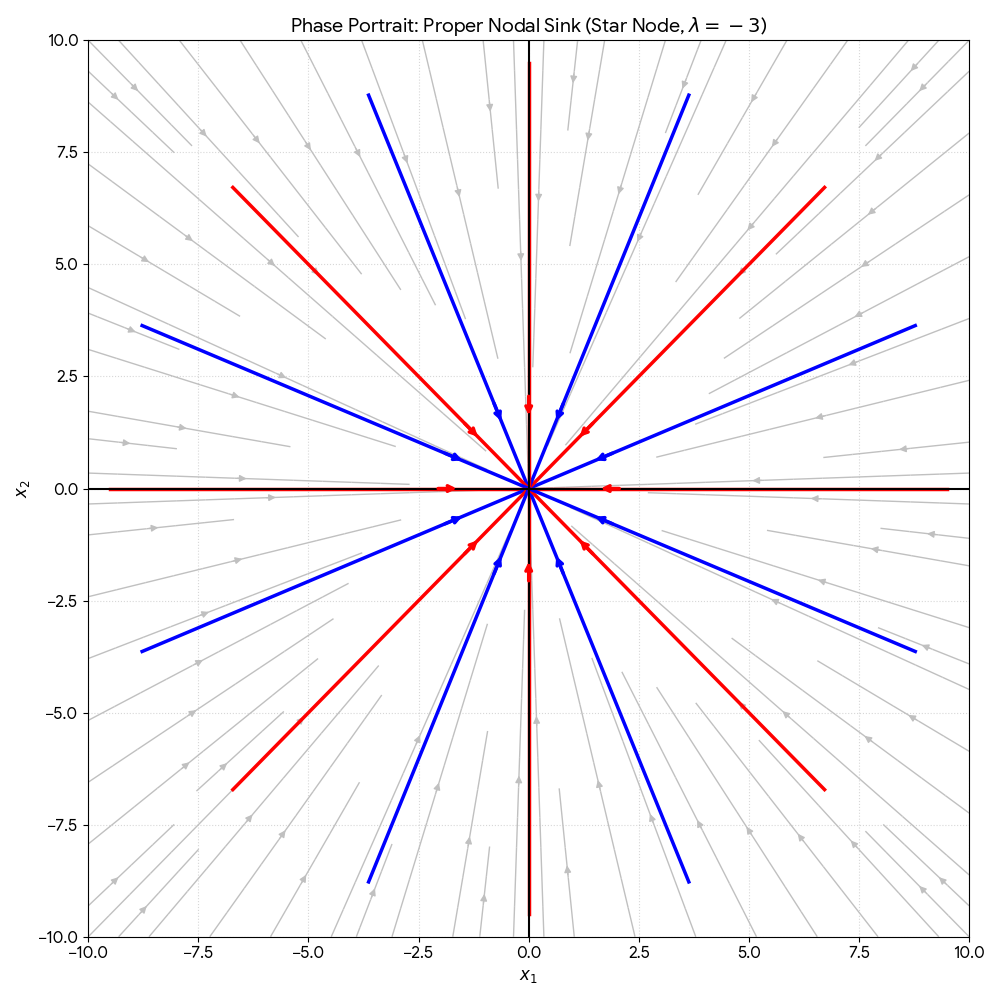
Case 1: Matrix \(\mathbf{A}\) has 2 Linearly Independent Eigenvectors (Complete)
Solve \(\vec{x}' = \begin{bmatrix} -3 & 0 \\ 0 & -3 \end{bmatrix} \vec{x}\).
\(\lambda = -3\) (multiplicity 2). Any vector is an eigenvector. Choose \(\vec{v}_1 = \begin{bmatrix} 1 \\ 0 \end{bmatrix}\) and \(\vec{v}_2 = \begin{bmatrix} 0 \\ 1 \end{bmatrix}\). General solution: \[\vec{x}(t) = \begin{bmatrix} C_1 \\ C_2 \end{bmatrix} e^{-3t}\]
Case 2: Matrix \(\mathbf{A}\) has only 1 Linearly Independent Eigenvector (Defective)
Recall Section 5.5 Example 2: \(\vec{x}' = \begin{bmatrix} 1 & -3 \\ 3 & 7 \end{bmatrix} \vec{x}\) has \(\lambda = 4\) (multiplicity 2). General solution: \[\vec{x}(t) = C_1 \begin{bmatrix} -3 \\ 3 \end{bmatrix} e^{4t} + C_2 \begin{bmatrix} -3t + 1 \\ 3t \end{bmatrix} e^{4t}\]
Analysis: If \(C_2 = 0\), the solution is the line \(x_1 = -x_2\). If \(C_2 \neq 0\), as \(t \to \infty\), the derivative \(\vec{x}'(t) \to \text{scalar multiple of } \vec{v}_1\). The line \(x_1 = -x_2\) is the tangent line to the solution curves.
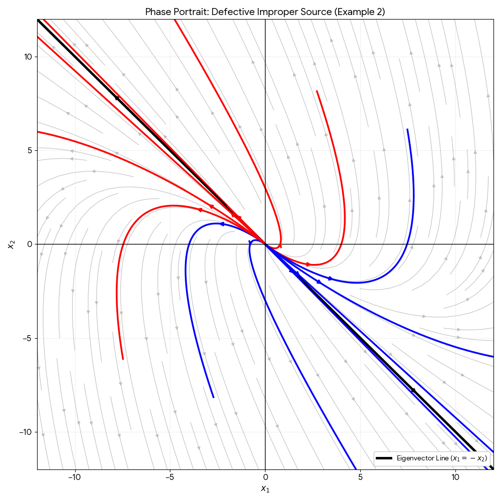
The origin is called an improper nodal source (unstable if \(\lambda > 0\)) or improper nodal sink (stable if \(\lambda < 0\)).
(III) Complex Conjugate Eigenvalues \(\lambda_{1,2} = p \pm iq\)
Case 1: \(p = 0\) (Purely Imaginary)
Solve \(\vec{x}' = \begin{bmatrix} 6 & -17 \\ 8 & -6 \end{bmatrix} \vec{x}\) with \(\vec{x}(0) = \begin{bmatrix} 4 \\ 2 \end{bmatrix}\).
Step 1: Eigenvalues. \(\det(\mathbf{A} - \lambda \mathbf{I}) = \lambda^2 + 100 = 0 \implies \lambda = \pm 10i\).
Step 2: Eigenvector for \(\lambda = 10i\). \(4a = (3 + 5i)b\). Let \(b = 4 \implies a = 3 + 5i\). Thus \(\vec{v} = \begin{bmatrix} 3+5i \\ 4 \end{bmatrix}\).
Step 3: Expansion. \(\vec{v}e^{\lambda t} = \begin{bmatrix} 3+5i \\ 4 \end{bmatrix} (\cos 10t + i \sin 10t) = \begin{bmatrix} 3\cos 10t - 5\sin 10t \\ 4\cos 10t \end{bmatrix} + i \begin{bmatrix} 5\cos 10t + 3\sin 10t \\ 4\sin 10t \end{bmatrix}\).
Step 4: General Solution:
Step 5: Particular Solution: Using \(\vec{x}(0) = \begin{bmatrix} 4 \\ 2 \end{bmatrix}\) yields \(C_1 = 1/2, C_2 = 1/2\). Resulting in:
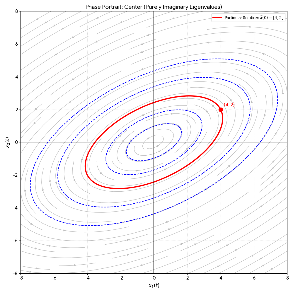
The solution curve is an ellipse rotated by \(\alpha = \arctan(3/4)\). The origin is called a center. It is stable, but not asymptotically stable.
Case 2: \(p \neq 0\) (Spiral Points)
From Section 5.2 Example 4: \(\lambda = 4 \pm 3i\). The general solution is \(x_1(t) = e^{4t}(C_1\cos 3t + C_2\sin 3t)\) and \(x_2(t) = e^{4t}(C_1\sin 3t - C_2\cos 3t)\). As \(t \to \infty, e^{4t} \to \infty\).
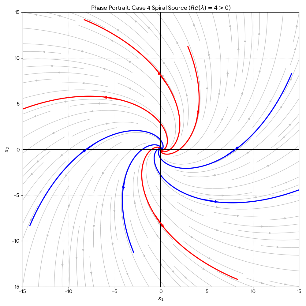
If \(p > 0\), the origin is called a spiral source (unstable) . If \(p < 0\), the origin is called a spiral sink (stable).
Summary of Classification
| Eigenvalues (\(\lambda_1, \lambda_2\)) | Condition | Critical Point Type | Stability |
|---|---|---|---|
| Real, Distinct | \(\lambda_1 < 0 < \lambda_2\) | Saddle Point | Unstable |
| Real, Distinct | \(\lambda_1 < \lambda_2 < 0\) | Improper Nodal Sink | Stable |
| Real, Distinct | \(0 < \lambda_1 < \lambda_2\) | Improper Nodal Source | Unstable |
| Repeated Real | Complete | Proper Nodal Sink (\(\lambda < 0\)) / Source (\(\lambda > 0\)) | Stable / Unstable |
| Repeated Real | Defective | Improper Nodal Sink (\(\lambda < 0\)) / Source (\(\lambda > 0\)) | Stable / Unstable |
| Complex Conjugate \(p \pm iq\) | \(p = 0\) | Center | Stable (not asym.) |
| Complex Conjugate \(p \pm iq\) | \(p < 0\) | Spiral Sink | Stable |
| Complex Conjugate \(p \pm iq\) | \(p > 0\) | Spiral Source | Unstable |
Stability Classifications
- Stable: Trajectories that start near the equilibrium point remain near it for all \(t > 0\).
- Asymptotically Stable: Trajectories that start near the equilibrium point approach the origin as \(t \to \infty\).
- Unstable: Trajectories that start near the equilibrium point move away from it.
Classification of Nodes
- Proper Node (Star Node): Occurs when there is a repeated eigenvalue with two linearly independent eigenvectors. Every trajectory is a straight line through the origin.
- Improper Node: Occurs when eigenvalues have the same sign (either distinct or repeated defective). Most trajectories are tangent to a specific straight line through the origin.