Review: The Unit Step Function
Recall from Section 7.1, the shifted unit step function \(u_a(t)\) is defined as:
If \(a = 0\), we have the standard unit step function \(u(t)\). The function \(u_a(t)\) is a piecewise function with a jump at \(t=a\).
Any piecewise continuous function \(f(t)\) can be written in terms of \(u_a(t)\) with different values of \(a\).
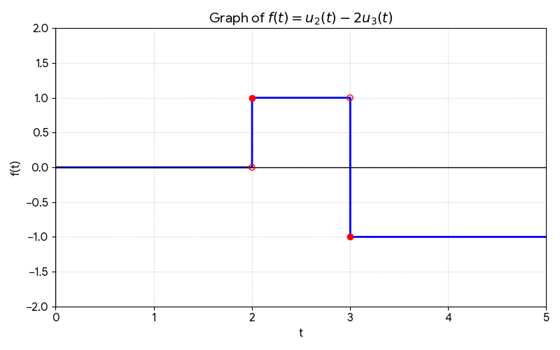
Sketch the graph of \( f(t) = u_2(t) - 2u_3(t) \) for \( t \ge 0 \).
Solution: We analyze the value of \(f(t)\) across different intervals based on the jumps at \(t=2\) and \(t=3\):
- For \(0 \le t < 2\): \( f(t) = 0 - 2(0) = 0 \)
- For \(2 \le t < 3\): \( f(t) = 1 - 2(0) = 1 \) (jump up 1 unit at \(t=2\))
- For \(t \ge 3\): \( f(t) = 1 - 2(1) = -1 \) (jump down 2 units at \(t=3\))
The function \(f(t)\) has two jumps: at \(t=2\) and \(t=3\).
Recall the Laplace transform of the unit step function:
Multiplication of the transform of \(u(t)\) by \(e^{-as}\) corresponds to a translation \(t \to t-a\).
(I) Translation on the t-axis
Theorem 1: Translation on the t-axis
If \( \mathcal{L}\{f(t)\} = F(s) \) exists for \( s > c \), then:
And inversely:
Find \( \mathcal{L}\{g(t)\} \) if \( g(t) = \begin{cases} 0 & \text{if } t < 3 \\ t^2 & \text{if } t \ge 3 \end{cases} \).
Solution: We can write \( g(t) = u(t-3)f(t-3) \). Since \( f(t-3) = t^2 \), we must find \( f(t) \):
Applying Theorem 1:
Find \( \mathcal{L}\{f(t)\} \) if \( f(t) = \begin{cases} \sin t & \text{if } 0 \le t \le 3\pi \\ 0 & \text{if } t > 3\pi \end{cases} \).
Solution: Express \( f(t) \) using unit step functions:
Now, take the Laplace transform:
Find \( \mathcal{L}\{f(t)\} \) if \( f(t) = \begin{cases} \sin(2t) & \text{if } \pi \le t \le 2\pi \\ 0 & \text{if } t < \pi \text{ or } t > 2\pi \end{cases} \).
Solution: Express \( f(t) \) using unit step functions:
Now, take the Laplace transform:
Find \( \mathcal{L}\{f(t)\} \) for \( f(t) = \begin{cases} t-1 & \text{if } t < 2 \\ 3-t & \text{if } 2 \le t \le 3 \\ 0 & \text{if } t > 3 \end{cases} \).
Solution: Express \( f(t) \) using unit step functions. The function starts as \(t-1\). At \(t=2\), we need to add a term to make it \(3-t\). At \(t=3\), we need to add a term to make it \(0\).
Now, take the Laplace transform:
Find \( \mathcal{L}^{-1}\{F(s)\} \) for \( F(s) = e^{-3s}\frac{s+1}{s^2-8s+20} \).
Solution: First, complete the square in the denominator: \(s^2 - 8s + 20 = (s-4)^2 + 4 = (s-4)^2 + 2^2\).
The inverse transform of the bracketed terms are \(e^{4t}\cos(2t)\) and \(\frac{5}{2}e^{4t}\sin(2t)\). The \(e^{-3s}\) factor means we apply the translation \(t \to t-3\) and multiply by \(u(t-3)\).
Find the Laplace transform of \( f(t) = \begin{cases} 0 & t < 1 \\ t^2 e^{2t} & t \ge 1 \end{cases} \).
Solution: Express \( f(t) \) using a unit step function:
Now take the Laplace transform of each term using the translation theorem:
(II) Transforms of Periodic Functions
\( f(t) \) is defined to be periodic if there is a number \( P > 0 \) such that \( f(t+P) = f(t) \) for all \( t \ge 0 \). The least positive value of \( P \) is called the period of \( f \).
Theorem 2: Transforms of Periodic Functions
Let \( f(t) \) be periodic with period \( P \) and piecewise continuous for \( t \ge 0 \). Then the transform \( F(s) = \mathcal{L}\{f(t)\} \) exists for \( s > 0 \) and is given by: