Review
In previous lessons, we solved equations of the form:
Now consider \(\frac{dy}{dx} = f(x, y)\). This involves both the independent variable \(x\) and the dependent variable \(y\). While direct integration can be difficult, graphical and numerical methods are used to construct approximate solutions that suffice for many practical purposes.
Recall that \(f'(a)\) is the slope of the tangent line to the graph of \(y=f(x)\) at \(x=a\).
(I) Slope Field and Graphical Solutions
The derivative \(y'\) represents the slope. At each point \((x, y)\) of the \(xy\)-plane, the value of \(f(x, y)\) determines the slope \(m = f(x, y)\). A solution of the D.E. is a differentiable function whose graph \(y = y(x)\) has this "correct slope" at each point through which it passes: \(y'(x) = f(x, y(x))\)
We draw short line segments having the proper slope \(m = f(x, y)\). All these line segments constitute a slope field or direction field for \(y' = f(x, y)\). A solution curve is simply a curve in the \(xy\)-plane whose tangent line at each point \((x, y)\) has slope \(m = f(x, y)\).
Construct a slope field for the D.E. \(y' = x - y\) and use it to sketch an approximate solution curve that passes through the point \((-4, 4)\).
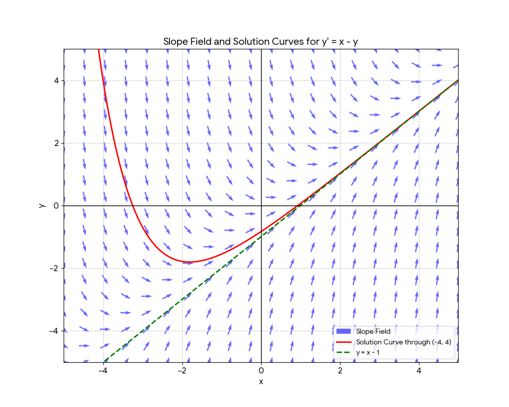
Slope field and solution curve for \(y' = x - y\). The solution through \((-4, 4)\) approaches the line \(y = x - 1\).
\(\frac{dy}{dx} = Ky\).
- \(K\) determines the direction of increase / decrease of \(y(x)\).
- \(|K|\) determines the rate of change of \(y(x)\).
- Actually \(y(x) = Ce^{Kx}\).
- For \(K = 2, 0.5\), the solution increases.
- For \(K = -1, -3\), \(y(x) \to 0\) as \(x \to \infty\).
(II) Application of Slope Field
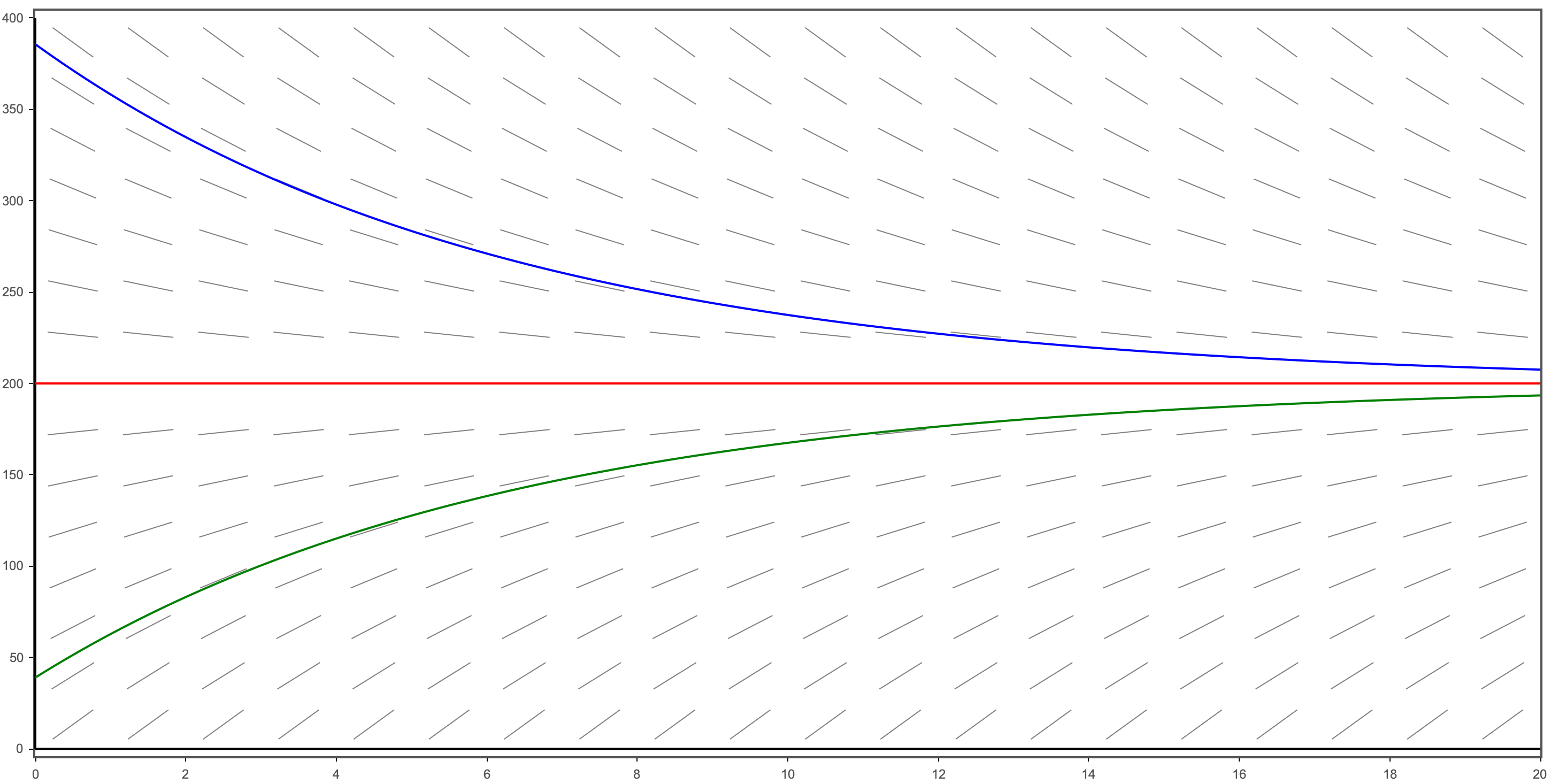
Consider air resistance proportional to velocity \(v\), where \(K = 0.16\):\(\frac{dv}{dt} = g - kv = 32 - 0.16v\)
Suppose you throw a baseball straight downward from a helicopter hovering at an altitude of 3000 ft. You wonder whether someone standing on the ground below could conceivably catch it.
For the differential equation \(\frac{dv}{dt} = 32 - 0.16v\), the direction field behaves as follows:
- The Equilibrium Line: At the value \(v = 200\), the slope segments are perfectly horizontal because \(\frac{dv}{dt} = 0\).
- Region Above \(v = 200\): The slope segments point downward (negative slope) because \(32 - 0.16v\) becomes negative when \(v > 200\).
- Region Below \(v = 200\): The slope segments point upward (positive slope) because \(32 - 0.16v\) is positive when \(v < 200\).
- Convergence: Any solution curve will "funnel" toward the horizontal line \(v = 200\), which represents the terminal velocity.
Given \(60 \text{ mi/h} = 88 \text{ ft/s}\), the terminal velocity is approximately \(136.36 \text{ mi/h}\).
Conclusion: Perhaps a catcher accustomed to \(100\) mi/h fastballs would have some chance of fielding this speeding ball.
Another application: Logistic D.E. \(\frac{dP}{dt} = kP(M - P)\).
(III) Existence and Uniqueness of Solutions
(a) Failure of Existence:
I.V.P. \(y' = \frac{1}{x}, y(0) = 0\). The function is discontinuous at \(x = 0\). \(y(x) = \ln(x) + C\) is undefined at \(x = 0\).
(b) Failure of Uniqueness:
\(f(x, y) = 2\sqrt{y}\). \(D_y f(x, y) = \frac{1}{\sqrt{y}}\) is discontinuous at \(y = 0\). I.V.P. \(y' = 2\sqrt{y}, y(0) = 0\). Both \(y_1(x) = x^2\) and \(y_2(x) \equiv 0\) are solutions.
Theorem 1: Existence and Uniqueness of Solutions
Suppose that both the function \(f(x, y)\) and its partial derivative \(D_y f(x, y)\) are continuous on some rectangle \(R\) in the \(xy\)-plane that contains the point \((a, b)\) in its interior. Then, for some open interval \(I\) containing the point \(a\), the I.V.P.:
has one and only one solution that is defined on the interval \(I\).
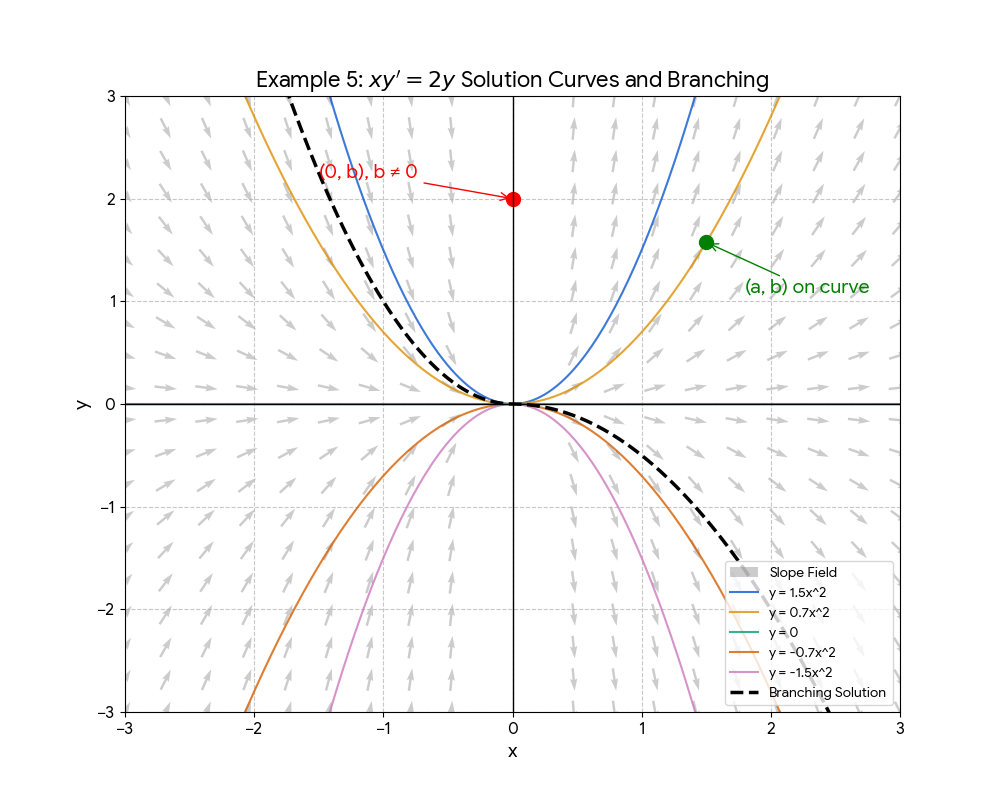
Consider the I.V.P. \(x\frac{dy}{dx} = 2y, y(a) = b\).
(a) Show that \(y(x) = Cx^2\) satisfies the D.E.:
\(L.H.S. = x \cdot (2Cx) = 2Cx^2 = 2y = R.H.S.\)
(b) Analyze existence and uniqueness:
\(f(x, y) = \frac{2y}{x}\) and \(D_y f(x, y) = \frac{2}{x}\). Both are continuous everywhere except at \(x = 0\).
| Condition | Outcome |
|---|---|
| If \(a \neq 0\) | The I.V.P. has a unique sol. near \((a, b)\) by Thm 1. |
| If \(a = 0, b = 0\) | Infinitely many solutions branch at the origin. |
| If \(a = 0, b \neq 0\) | No sol. exists through \((0, b)\). |
Remark: Thm 1 only guarantees uniqueness near the initial point. Solution curves can branch later. For example, \(y(x) = x^2\) for \(x \le 0\) and \(y(x) = Cx^2\) for \(x > 0\) is also a valid solution.