Lecture 5 & 6: Sec 1.5 Linear First-order Equations

(I) Linear 1st-order Equation, Integrating Factor

1st order equation: $\frac{dy}{dx} = f(x,y)$

The standard form of a linear 1st-order equation:

\frac{dy}{dx} + P(x)y = Q(x) \tag{*}

where $P(x)$ and $Q(x)$ are continuous on some interval on the x-axis.

We'd like to multiply both sides by a factor s.t. both sides could be recognized as derivatives.

\text{Integrating Factor: } \rho(x) = e^{\int P(x)dx}

$e^{\int P(x)dx} \frac{dy}{dx} + P(x)e^{\int P(x)dx}y = Q(x)e^{\int P(x)dx}$

Note that L.H.S. $= D_x [y(x)e^{\int P(x)dx}]$, we now have

D_x [y(x)e^{\int P(x)dx}]\ = Q(x)e^{\int P(x)dx}

Integrating both sides to get

y(x)e^{\int P(x)dx} = \int Q(x)e^{\int P(x)dx}dx + C

y(x) = e^{-\int P(x)dx} \left[\int Q(x)e^{\int P(x)dx}dx + C\right]

Remark: Method is more important than formula.

EXAMPLE 1

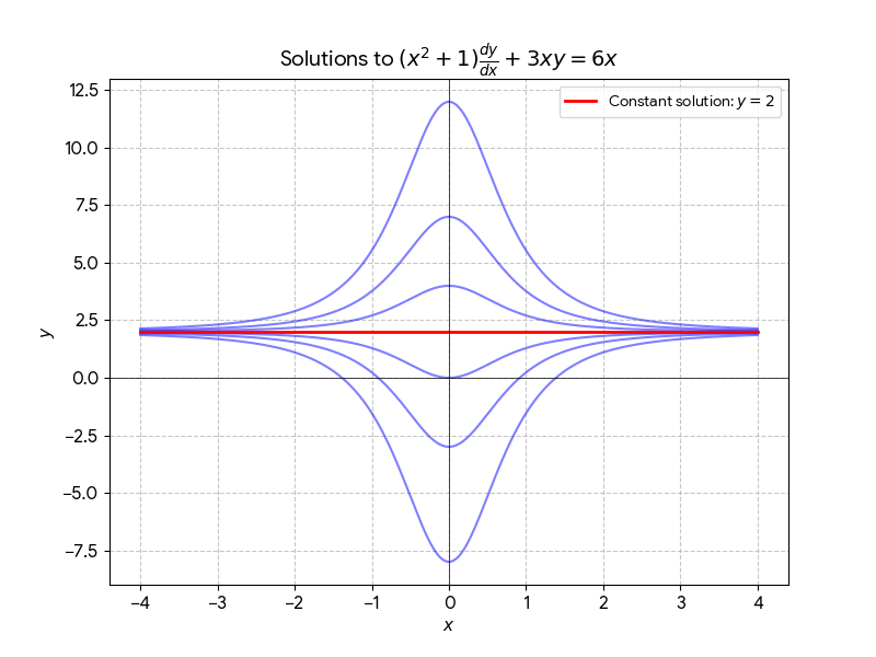
(1) Find the general solution of the D.E.: $$(x^2+1)\frac{dy}{dx} + 3xy = 6x $$

First, rewrite the first-order linear differential equation in standard form.

\frac{dy}{dx} + \frac{3x}{x^2+1}y = \frac{6x}{x^2+1}

$P(x) = \frac{3x}{x^2+1}$, $Q(x) = \frac{6x}{x^2+1}$

\rho = e^{\int \frac{3x}{x^2+1}dx} = e^{\frac{3}{2}\ln(x^2+1)} = (x^2+1)^{\frac{3}{2}}

Remark: When finding the integrating factor, there is no need to add +C, since any constant multiple of an integrating factor works.

$D_x [y(x^2+1)^{\frac{3}{2}}] = 6x(x^2+1)^{\frac{1}{2}}$

$y(x^2+1)^{\frac{3}{2}} = \int 6x(x^2+1)^{\frac{1}{2}}dx = 2(x^2+1)^{\frac{3}{2}} + C$

The general solution is $y(x) = 2 + C(x^2+1)^{-\frac{3}{2}}$.

(2) If $y(0)=2$, then find the particular sol.

$y(0) = 2 + C = 2 \implies C = 0$

$y(x) \equiv 2$ is the particular sol.

Constant solution can be described as an equilibrium solution.

In fact, if $ y(x) \equiv 2 $, then $ y'(x) = 0 $, meaning there is no rate of change and $ y $ remains constant.

Coordinate plane showing a family of solution curves converging toward the equilibrium solution y=2.

EXAMPLE 2

Solve the I.V.P.: $$xy' - 3y = x^3, \quad y(1)=10$$

First, rewrite in standard form:

y' - \frac{3}{x}y = x^2

$P(x) = -\frac{3}{x}$, $Q(x) = x^2$

Find the Integrating Factor:

\rho(x) = e^{\int -\frac{3}{x}dx} = e^{-3\ln x} = x^{-3}

$D_x(yx^{-3}) = x^{-3} \cdot x^2 = x^{-1}$

$yx^{-3} = \int x^{-1}dx = \ln|x| + C \implies y = x^3(\ln|x| + C)$

Applying initial condition $y(1) = 10$:

$y(1) = 1^3(0 + C) = 10 \implies C = 10$

The particular solution is $y(x) = x^3(\ln|x| + 10)$.

EXAMPLE 3

Solve the D.E. by regarding $y$ as the indep. variable rather than $x$: $$ (1 - 4xy^2) \frac{dy}{dx} = y^3 $$

Rewrite by taking the reciprocal:

$\frac{1 - 4xy^2}{y^3} = \frac{dx}{dy} \implies \frac{dx}{dy} + \frac{4}{y}x = \frac{1}{y^3}$

$P(y) = \frac{4}{y}$, $Q(y) = \frac{1}{y^3}$

Find the Integrating Factor:

$\rho(y) = e^{\int \frac{4}{y}dy} = e^{4\ln|y|} = y^4$

$D_y(y^4x) = y^4 \cdot \frac{1}{y^3} = y$

$y^4x = \int y \, dy = \frac{1}{2}y^2 + C$

The general solution is $x = \frac{1}{2}y^{-2} + Cy^{-4}$.

(II) Existence and Uniqueness Theorem

If $P(x)$ and $Q(x)$ are continuous on the open interval $I$, then antiderivatives $\int P(x)dx$ and $\int Q(x)dx$ exist on $I$. $y(x) = e^{-\int P(x)dx} \left[\int Q(x)e^{\int P(x)dx}dx + C\right]$ is a solution of the linear 1st-order equation $(*)$. If $y(x_0)=y_0$, there's a unique value of $C$.

Theorem 1: Existence and Uniqueness Theorem for the Linear First-Order Equation

If the functions $ P(x) $ and $ Q(x) $ are continuous on the open interval $ I $ containing $ x_0 $, then the I.V.P.

\frac{dy}{dx} + P(x)y = Q(x), \quad y(x_0) = y_0

has a unique solution $ y(x) $ on $ I $ given by formula (1) with an appropriate value of $ C $.

Remarks

Theorem 1 gives a solution on the entire interval $I$ for a linear differential equation, in contrast with theorems for general equations which may guarantee solutions only on a smaller interval.
Theorem 1 tells us that every solution of $(*)$ is included in the general solution. Thus, a linear 1st-order D.E. has no singular solutions.
To solve an I.V.P., the appropriate value of $C$ can be selected by writing the integrating factor as $\rho(x) = \exp(\int_{x_0}^{x} P(t)dt)$: $y(x) = \frac{1}{\rho(x)} [y_0 + \int_{x_0}^{x} \rho(t)Q(t)dt]$

EXAMPLE 4

Determine the interval on which the I.V.P. below has a unique solution: $$ (t+2)y' + y = \frac{1}{t-1}, \quad y(0) = \frac{1}{2} $$

First, rewrite in standard form:

y' + \frac{1}{t+2}y = \frac{1}{(t-1)(t+2)}

$P(t) = \frac{1}{t+2}$ and $Q(t) = \frac{1}{(t-1)(t+2)}$ are continuous when $t \neq -2$ and $t \neq 1$.

Possible intervals: $(-\infty, -2)$, $(-2, 1)$, and $(1, \infty)$.

Since the initial time $t_0 = 0$ is in the interval $(-2, 1)$, the unique solution exists on (-2, 1).

(III) Application: Mixture Problems

Consider a tank containing a solution of solute (like salt) and solvent (water). There are both inflow and outflow, and we want to compute the amount $x(t)$ of solute in the tank at time $t$.

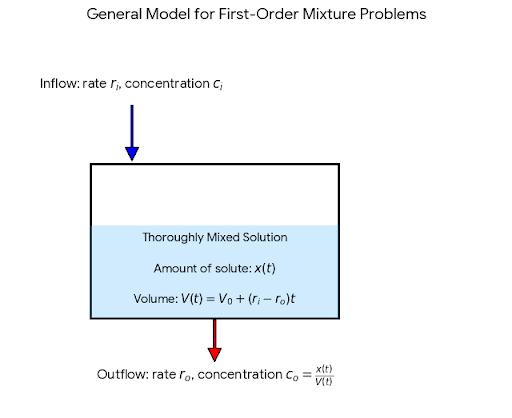
Diagram of a mixing tank showing inflow of brine and outflow of the perfectly mixed solution.

Inflow: constant rate $r_i$ (L/s), concentration $c_i$ (g/L).
Outflow: constant rate $r_o$ (L/s), concentration $c_o = \frac{x(t)}{V(t)}$ (g/L).
Volume: $V(t) = V_0 + (r_i - r_o)t$.

Set up a D.E. for $x(t)$ by balancing input and output rates:

\frac{dx}{dt} = (\text{input rate}) - (\text{output rate}) = r_i c_i - r_o c_o

\frac{dx}{dt} = r_i c_i - \frac{r_o}{V(t)}x

Remark: Understanding the process makes memorizing the formula easier.

EXAMPLE 5: Salt Tank Problem

A 120-gal tank initially contains 90 lb of salt dissolved in 90 gal of water. Brine with 2 lb/gal flows in at 4 gal/min. The mixture flows out at 3 gal/min. How much salt is in the tank when it's full?

$r_i = 4$ gal/min, $c_i = 2$ lb/gal.
$r_o = 3$ gal/min, $c_o = \frac{x(t)}{V(t)}$.
$V(t) = 90 + (4-3)t = 90 + t$.

\frac{dx}{dt} = 4 \cdot 2 - 3 \cdot \frac{x}{90+t} \implies \frac{dx}{dt} + \frac{3}{90+t}x = 8

Find the Integrating Factor:

$\rho(t) = e^{\int \frac{3}{90+t}dt} = (90+t)^3$

$D_t [x \cdot (90+t)^3] = 8(90+t)^3$

$x(90+t)^3 = \int 8(90+t)^3 dt = 2(90+t)^4 + C$

Applying $x(0) = 90$: $90 \cdot 90^3 = 2 \cdot 90^4 + C \implies C = -90^4$.

$x(t) = 2(90+t) - \frac{90^4}{(90+t)^3}$

Tank is full when $V(t) = 120 \implies t = 30$.

$x(30) = 2(120) - \frac{90^4}{120^3} \approx 202 \text{ lb}$.

EXAMPLE 6

Assume that Lake Erie has a volume of $480 \text{ km}^3$, and that its rate of inflow from Lake Huron and outflow to Lake Ontario are both $350 \text{ km}^3/\text{year}$. Suppose that at $t = 0$, the pollutant concentration of Lake Erie is 5 times that of Lake Huron. If the outflow is perfectly mixed lake water, how long will it take to reduce the pollution concentration in Lake Erie to twice that of Lake Huron?

Setup:

$V = 480 \text{ km}^3$ (fixed volume since $r_i = r_o$)
$r_i = 350 \text{ km}^3/\text{year}$
$r_o = 350 \text{ km}^3/\text{year}$
$c_i = c$ (the pollutant concentration of Lake Huron)
$x(0) = 5cV$ (initial amount of pollutant)

Question: When is $x(t) = 2cV$?

$\frac{dx}{dt} = r_i c_i - r_o c_o = 350c - 350\frac{x}{V}$

\frac{dx}{dt} + \left(\frac{350}{V}\right)x = 350c

Find the Integrating Factor:

$\rho(t) = e^{\int \frac{350}{V} dt} = e^{\frac{350}{V}t}$

Apply the Integrating Factor:

$D_t(x e^{\frac{350}{V}t}) = 350 c e^{\frac{350}{V}t}$

$x e^{\frac{350}{V}t} = \int 350 c e^{\frac{350}{V}t} dt = cV e^{\frac{350}{V}t} + K$

Solve for $x(t)$:

$x(t) = cV + K e^{-\frac{350}{V}t}$

Use Initial Condition:

$x(0) = cV + K = 5cV \implies K = 4cV$

Solve for target time $t$:

$x(t) = cV + 4cV e^{-\frac{350}{V}t} = 2cV$

$4cV e^{-\frac{350}{V}t} = cV \implies e^{-\frac{350}{V}t} = \frac{1}{4}$

$\frac{350}{V}t = \ln 4$

$t = \ln 4 \cdot \frac{480}{350} \approx 1.901 \text{ years}$