Lecture 9: Sec 2.1 Population Models

Introduction

In Section 1.4, we introduced the exponential differential equation: $\frac{dP}{dt} = kP$ with $P(t) = P_0 e^{kt}$

This serves as a mathematical model for natural population growth resulting from a constant birth rate $\beta$ and a constant death rate $\delta$, where $k = \beta - \delta$ and $P_0 = P(0)$.

Suppose that the population changes only by the occurrence of births and deaths (no immigration, etc.). We consider $P(t)$ as a continuous approximation to the actual population. The general population equation is:

$$\frac{dP}{dt} = (\beta(t) - \delta(t))P$$

(I) Bounded Population and the Logistic Equation

It is often observed that the birth rate decreases as the population itself increases. For example, let $\beta = \beta_0 - \beta_1 P$ (a decreasing function of $P$) while the death rate $\delta = \delta_0$ remains constant.

\frac{dP}{dt} = (\beta_0 - \beta_1 P - \delta_0)P \implies \frac{dP}{dt} = aP - bP^2

where $a = \beta_0 - \delta_0$ and $b = \beta_1 > 0$. This is called the Logistic Equation if $a > 0, b > 0$.

To relate the behavior of $P(t)$ to the value of parameters, we rewrite it as:

\frac{dP}{dt} = kP(M - P)

where $k = b > 0$ and $M = a/b$ are constants.

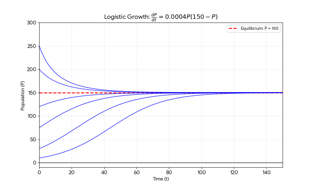
Example 1: Solve the Logistic Equation

Consider the equation: $$\frac{dP}{dt} = 0.0004P(150 - P), \quad P(0) = P_0$$

1. Separate the variables and integrate:

$$\int \frac{dP}{P(150 - P)} = \int 0.0004 \, dt$$

2. Use partial fraction decomposition:

Note that $ \frac{1}{P(150 - P)} = \frac{1/150}{P} + \frac{1/150}{150 - P} $. Multiplying the equation by 150 gives:

$$\int \left( \frac{1}{P} + \frac{1}{150 - P} \right) dP = \int (150 \times 0.0004) \, dt$$

$$\int \left( \frac{1}{P} + \frac{1}{150 - P} \right) dP = \int 0.06 \, dt$$

3. Perform the integration:

$$\ln|P| - \ln|150 - P| = 0.06t + C_1$$

$$\ln \left| \frac{P}{150 - P} \right| = 0.06t + C_1$$

4. Solve for the ratio:

$$\frac{P}{150 - P} = e^{0.06t + C_1} = C e^{0.06t}$$

5. Apply initial condition $ P(0) = P_0 $ to find $ C $:

$$\frac{P_0}{150 - P_0} = C e^{0} \implies C = \frac{P_0}{150 - P_0}$$

6. Final particular solution for $ P(t) $:

$$\frac{P}{150 - P} = \frac{P_0}{150 - P_0} e^{0.06t}$$

After algebraic rearrangement:

$$P(t) = \frac{150 P_0}{P_0 + (150 - P_0)e^{-0.06t}}$$

7. Equilibrium analysis:

$$\lim_{t \to \infty} P(t) = 150$$

When $ P = 150 $, $ \frac{dP}{dt} = 0 $, so $ P \equiv 150 $ is an equilibrium solution. All solution curves approach this line as an asymptote.

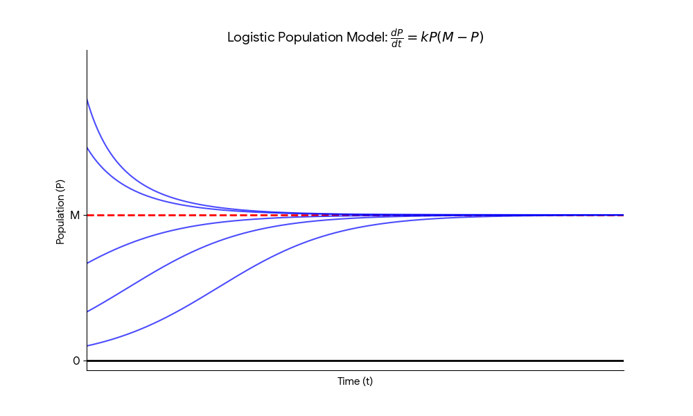
A coordinate plane with population P on the vertical axis and time t on the horizontal axis. A dashed horizontal line is at P=150. Curves starting below 150 rise and level off at the line. Curves starting above 150 fall and level off at the line.

(II) Limiting Population and Carrying Capacity

The solution to the logistic equation $\frac{dP}{dt} = kP(M-P)$ with $P(0) = P_0$ is given by:

P(t) = \frac{M P_0}{P_0 + (M - P_0)e^{-kMt}}

$P(t) \equiv M$ is called the equilibrium population. We analyze the behavior based on the initial population $P_0$:

If $P_0 > M$: Then $P' < 0$. In this case, $M - P_0$ is a negative number, which leads to: $P(t) = \frac{M P_0}{P_0 + (\text{neg. number})} > \frac{M P_0}{P_0} = M$ The population decreases steadily and approaches $M$ from above.
If $0 < P_0 < M$: Then $P' > 0$. The population increases steadily and approaches $M$ from below.

In any case, the population eventually stabilizes:

\lim_{t \to \infty} P(t) = M

$M$ is defined as the limiting population or carrying capacity.

A graph of the logistic population model showing time on the x-axis and population P on the y-axis. A horizontal dashed line is labeled M (stable equilibrium) and a solid line at 0. Curves from below M rise toward it in an S-shape; curves from above M decline toward it. — Logistic Model: dP/dt = kP(M - P)

Ex2: Rabbit Population Model

Consider a population $ P(t) $ satisfying the logistic equation: $$\frac{dP}{dt} = aP - bP^2, \quad P(0) = P_0$$

$ B = aP $ is the time rate at which births occur.
$ B_0 = aP_0 $ is the birth rate at $ t = 0 $.
$ D = bP^2 $ is the time rate at which deaths occur.
$ D_0 = bP_0^2 $ is the death rate at $ t = 0 $.

Problem: If the initial population is 120 rabbits and there are 8 births per month and 6 deaths per month occurring at time $ t = 0 $, how many months does it take for $ P(t) $ to reach 95% of the limiting population $ M $?

1. Find the Limiting Population (M): $$M = \frac{a}{b} = \frac{B_0 / P_0}{D_0 / P_0^2} = \frac{B_0 P_0}{D_0}$$ Using the given values: $$M = \frac{8 \times 120}{6} = 160$$

2. Determine the constant $ k $: $$k = \frac{b}{120} = \frac{D_0 / P_0^2}{120} \text{ (from } b = \frac{D_0}{P_0^2} \text{)}$$ $$k = \frac{6}{120^2} = \frac{1}{2400}$$

3. Calculate the time $ t $: Using the logistic solution formula: $$P(t) = \frac{M P_0}{P_0 + (M - P_0)e^{-kMt}} = 0.95M$$ Substituting $ P_0 = 120, M = 160 $, and $ kM = \frac{160}{2400} = \frac{1}{15} $: $$\frac{120M}{120 + (160 - 120)e^{-\frac{1}{15}t}} = 0.95M$$

Result: $$t \approx 27.69 \text{ months}$$

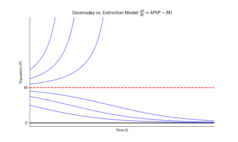
(III) Doomsday Versus Extinction

Consider animals that rely on chance encounters for reproduction. Encounters occur at a rate proportional to $P/2 \times P/2$, hence proportional to $P^2$.

\frac{dP}{dt} = kP^2 - \delta P = kP(P - M) \text{ where } M = \delta/k

If $P_0 > M$: $P' > 0$, leads to a population explosion.
If $P_0 < M$: $P' < 0$, leads to population extinction.

$M$ is called the threshold population. The outcome depends critically on whether $P_0$ is above or below $M$.

A coordinate plane showing population P over time t. A dashed horizontal line is labeled M, and a solid horizontal line is at 0. Curves starting between 0 and M slope downward toward 0 (Extinction). Curves starting above M slope sharply upward toward infinity (Doomsday). — Figure: Doomsday vs. Extinction Model where M is the unstable equilibrium threshold.

Extra Example: Rumor Spreading

Suppose half of a logistic population of 100,000 have heard a rumor at $t=0$. The number of those who heard it is increasing at a rate of 1000 per day. How long to spread to 80%?

Setup: $M = 100,000$, $P(0) = 50,000$, $P'(0) = 1000$.

$P' = kP(M - P) \implies 1000 = k(50,000)(100,000 - 50,000) \implies k = \frac{1}{2,500,000}$.

Solve for $P(t) = 0.8M = 80,000$:

$$\frac{100,000}{1 + e^{-0.04t}} = 80,000 \implies \frac{1}{1 + e^{-0.04t}} = 0.8 \implies t \approx 34.66 \text{ days.}$$