Introduction
This section connects equations involving vectors to ordinary systems of equations.
Definition: Column Vector
A matrix with only one column is called a column vector, or simply a vector.
(I) Vectors in \(\mathbb{R}^2\)
For example, \(\vec{u} = \begin{bmatrix} 2 \\ -3 \end{bmatrix}\) and \(\vec{v} = \begin{bmatrix} 0.2 \\ \sqrt{3} \end{bmatrix}\) are vectors in \(\mathbb{R}^2\). In general, a vector \(\vec{w} = \begin{bmatrix} w_1 \\ w_2 \end{bmatrix}\) where \(w_1\) and \(w_2\) are any real numbers is an element of \(\mathbb{R}^2\), the set of all vectors with two entries.
Vector Operations
Let \(\vec{u} = \begin{bmatrix} u_1 \\ u_2 \end{bmatrix}\) and \(\vec{v} = \begin{bmatrix} v_1 \\ v_2 \end{bmatrix}\) be two vectors in \(\mathbb{R}^2\).
- Equality: \(\vec{u} = \vec{v}\) if and only if \(u_1 = v_1\) and \(u_2 = v_2\).
- Sum: \(\vec{u} + \vec{v} = \begin{bmatrix} u_1 + v_1 \\ u_2 + v_2 \end{bmatrix}\).
- Scalar Multiplication: Given a scalar \(c\), \(c\vec{u} = \begin{bmatrix} c u_1 \\ c u_2 \end{bmatrix}\).
Geometric Description of \(\mathbb{R}^2\)
Consider a rectangular coordinate system plane. We can identify a geometric point \((a, b)\) with the vector \(\begin{bmatrix} a \\ b \end{bmatrix}\). Thus, we may regard \(\mathbb{R}^2\) as the set of all points in the plane. We can represent vectors as points or as arrows from the origin. Note that while \(\begin{bmatrix} 2 \\ -3 \end{bmatrix}\) is often written as \((2, -3)\) for convenience, the matrix \(\begin{bmatrix} 2 & -3 \end{bmatrix}\) is not the same as the column vector.
Parallelogram Rule for Addition
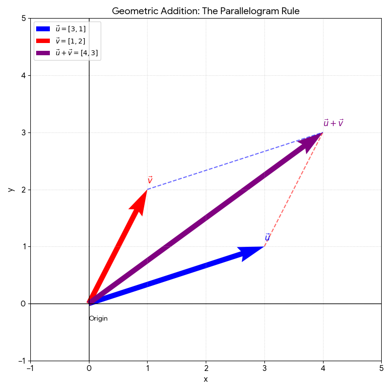
If \(\vec{u}\) and \(\vec{v}\) in \(\mathbb{R}^2\) are represented as points in the plane, then \(\vec{u} + \vec{v}\) corresponds to the fourth vertex of the parallelogram whose other three vertices are \(\vec{u}\), \(\vec{v}\), and the origin \(\vec{0}\).
Let \(\vec{u} = \begin{bmatrix} 1 \\ 1 \end{bmatrix}\) and \(\vec{v} = \begin{bmatrix} -6 \\ 1 \end{bmatrix}\). Find and display \(2\vec{u}\), \(-\frac{1}{2}\vec{v}\), and \(2\vec{u} - \frac{1}{2}\vec{v}\).
Solution:
- \(2\vec{u} = \begin{bmatrix} 2 \\ 2 \end{bmatrix}\). Geometrically, the arrow for \(2\vec{u}\) is twice as long as \(\vec{u}\) and points in the same direction.
- \(-\frac{1}{2}\vec{v} = \begin{bmatrix} 3 \\ -0.5 \end{bmatrix}\). The arrow points in the opposite direction of \(\vec{v}\).
- \(2\vec{u} - \frac{1}{2}\vec{v} = \begin{bmatrix} 2 + 3 \\ 2 - 0.5 \end{bmatrix} = \begin{bmatrix} 5 \\ 1.5 \end{bmatrix}\).
(II) Vectors in \(\mathbb{R}^n\)
For any positive integer \(n\), \(\mathbb{R}^n\) denotes the set of all lists (or ordered n-tuples) of \(n\) real numbers, usually written as \(n \times 1\) column matrices:
The zero vector, denoted by \(\vec{0}\), is the vector whose entries are all zeros. Operations in \(\mathbb{R}^n\) are defined entry by entry, just as in \(\mathbb{R}^2\).
Algebraic Properties of \(\mathbb{R}^n\)
For all \(\vec{u}, \vec{v}, \vec{w}\) in \(\mathbb{R}^n\) and all scalars \(c\) and \(d\):
- \(\vec{u} + \vec{v} = \vec{v} + \vec{u}\)
- \((\vec{u} + \vec{v}) + \vec{w} = \vec{u} + (\vec{v} + \vec{w})\)
- \(\vec{u} + \vec{0} = \vec{0} + \vec{u} = \vec{u}\)
- \(\vec{u} + (-\vec{u}) = -\vec{u} + \vec{u} = \vec{0}\), where \(-\vec{u} = (-1)\vec{u}\)
- \(c(\vec{u} + \vec{v}) = c\vec{u} + c\vec{v}\)
- \((c + d)\vec{u} = c\vec{u} + d\vec{u}\)
- \(c(d\vec{u}) = (cd)\vec{u}\)
- \(1\vec{u} = \vec{u}\)
(III) Linear Combinations and Existence Problem
Definition: Linear Combination
Given vectors \(\vec{v}_1, \vec{v}_2, \dots, \vec{v}_p\) in \(\mathbb{R}^n\) and scalars \(c_1, c_2, \dots, c_p\), the vector \(\vec{Y}\) defined by:
is called a linear combination of \(\vec{v}_1, \dots, \vec{v}_p\) with weights \(c_1, \dots, c_p\). The weights can be any real numbers, including zero.
Identify selected linear combinations of \(\vec{v}_1 = \begin{bmatrix} -1 \\ 1 \end{bmatrix}\) and \(\vec{v}_2 = \begin{bmatrix} 2 \\ 1 \end{bmatrix}\) using a coordinate grid.
Interactive Skewed Grid
Basis Vectors: v₁ = [-1, 1] (Solid Blue) and v₂ = [2, 1] (Solid Teal)
Definition of Span
If \(\vec{v}_1, \dots, \vec{v}_p\) are in \(\mathbb{R}^n\), then Span\(\{\vec{v}_1, \dots, \vec{v}_p\}\) is the set of all linear combinations of those vectors. It is the collection of vectors \(c_1\vec{v}_1 + \dots + c_p\vec{v}_p\) with \(c_1, \dots, c_p\) as scalars. This is also called the subset of \(\mathbb{R}^n\) spanned (generated) by \(\vec{v}_1, \dots, \vec{v}_p\).
Note: While \(\{\vec{v}_1, \dots, \vec{v}_p\}\) is a set containing only \(p\) vectors, if at least one vector is non-zero, then the Span is a set containing infinitely many vectors. The zero vector \(\vec{0}\) is always in the Span.
Equivalent Questions
The following questions are different ways of asking the same thing:
- Is \(\vec{b}\) in Span\(\{\vec{v}_1, \dots, \vec{v}_p\}\)?
- Can \(\vec{b}\) be generated as a linear combination of \(\vec{v}_1, \dots, \vec{v}_p\)?
- Does the vector equation \(x_1\vec{v}_1 + \dots + x_p\vec{v}_p = \vec{b}\) have a solution?
- Does the linear system with the augmented matrix \([\vec{v}_1 \dots \vec{v}_p \ | \ \vec{b}]\) have a solution?
Let \(\vec{a}_1 = \begin{bmatrix} 1 \\ -2 \\ -5 \end{bmatrix}\), \(\vec{a}_2 = \begin{bmatrix} 2 \\ 5 \\ 6 \end{bmatrix}\), and \(\vec{b} = \begin{bmatrix} 7 \\ 4 \\ -3 \end{bmatrix}\). Determine whether \(\vec{b}\) is in the Span of \(\vec{a}_1\) and \(\vec{a}_2\). If yes, write \(\vec{b}\) as a linear combination.
Solution: Form the augmented matrix and reduce to Reduced Row Echelon Form:
We find that \(x_1 = 3\) and \(x_2 = 2\). Since the system is consistent, \(\vec{b}\) is in the Span. In fact, \(3\vec{a}_1 + 2\vec{a}_2 = \vec{b} \)
(IV) A Geometric Description of Span
Span of a Single Vector
If \(\vec{v}\) is a non-zero vector in \(\mathbb{R}^3\), then Span\(\{\vec{v}\}\) is the set of all scalar multiples of \(\vec{v}\). This is a line through the origin and \(\vec{v}\).
Span of Two Vectors
If \(\vec{u}\) and \(\vec{v}\) are vectors in \(\mathbb{R}^3\) that are not on the same line, then Span\(\{\vec{u}, \vec{v}\}\) is the collection of all linear combinations \(c_1\vec{u} + c_2\vec{v}\). Geometrically, this is a plane in \(\mathbb{R}^3\) containing \(\vec{u}\), \(\vec{v}\), and the origin.
Let \(\vec{a}_1 = \begin{bmatrix} 1 \\ -2 \\ 3 \end{bmatrix}\) and \(\vec{a}_2 = \begin{bmatrix} 5 \\ -13 \\ -3 \end{bmatrix}\). These vectors define a plane through the origin in \(\mathbb{R}^3\). Is \(\vec{b} = \begin{bmatrix} -3 \\ 8 \\ 1 \end{bmatrix}\) in that plane?
Solution: We check if the vector equation \(x_1\vec{a}_1 + x_2\vec{a}_2 = \vec{b}\) has a solution.
The last row represents the equation \(0 = -2\), which is never true. The system has no solution.
Conclusion: \(\vec{b}\) is not in the plane spanned by \(\vec{a}_1\) and \(\vec{a}_2\).