Recall:
Theorem 2 (Existence and Uniqueness Theorem)
Existence: A linear system is consistent if and only if the rightmost column of the augmented matrix is not a pivot column. That is, if and only if an echelon form has no row of the form:
with \(b \neq 0\).
Uniqueness: If it's consistent, then the solution set contains:
- a unique solution when there is no free variable.
- infinitely many solutions when there is at least one free variable.
(I) Homogeneous Linear System
Definition
A linear system is said to be homogeneous if it can be written in the form \(A\vec{x}=\vec{0}\), where \(A\) is an \(m \times n\) matrix and \(\vec{0} \in \mathbb{R}^m\).
It always has at least one solution, namely \(\vec{x}=\vec{0}\). This is called the trivial solution, the zero vector in \(\mathbb{R}^n\).
Uniqueness question: Does \(A\vec{x}=\vec{0}\) have a nontrivial solution?
Existence and uniqueness theorem tells us:
Proposition
\(A\vec{x}=\vec{0}\) has a nontrivial solution if and only if the equation has at least one free variable.
Determine if the following homogeneous equation has a nontrivial solution. Then describe the solution set.
Solution: We can use either the coefficient matrix or the augmented matrix for homogeneous Linear Systems.
Translating this back to equations:
Writing the solution in parametric vector form:
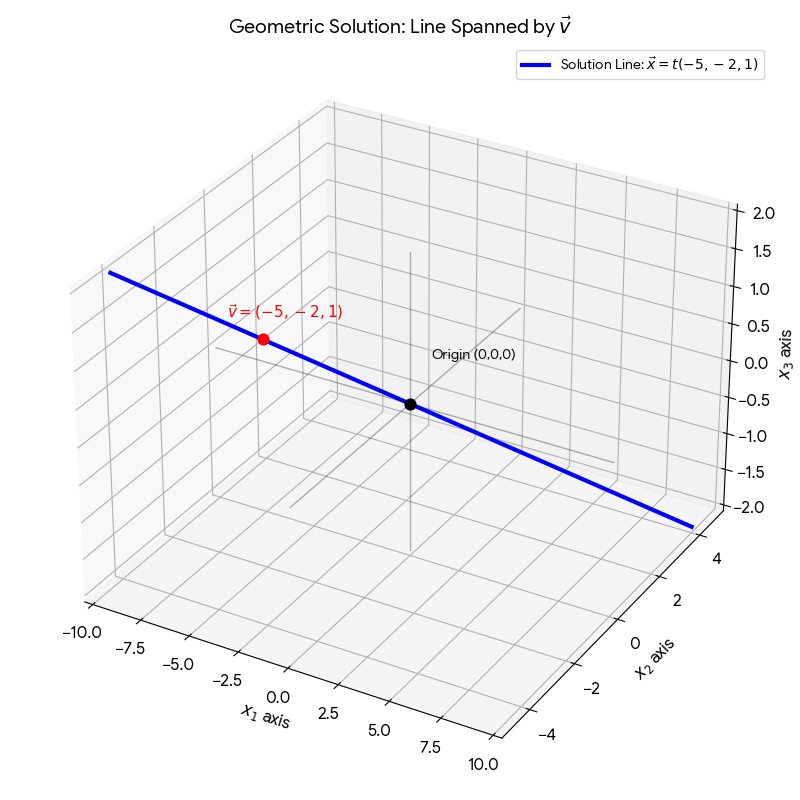
Description: The solution set is a line through \(\vec{0}\) and \(\vec{v}\) in \(\mathbb{R}^3\). This represents \(\text{Span}\{\vec{v}\}\).
A single Linear equation can be treated as a very simple system of equations. Describe the solution of the homogeneous "system":
Solution: There is no need for matrix notation. Solve for the basic variable \(x_1\) in term of the free variables \(x_2\) and \(x_3\).
In parametric vector form:
Description: Every solution is a linear combination of \(\vec{u}\) and \(\vec{v}\), i.e., \(\text{Span}\{\vec{u}, \vec{v}\}\). Since neither \(\vec{u}\) nor \(\vec{v}\) is a scalar multiple of the other, the solution set is a plane through \(\vec{u}\), \(\vec{v}\) and the origin in \(\mathbb{R}^3\).
Conclusion
The solution set of a homogeneous equation \(A\vec{x}=\vec{0}\) can always be expressed explicitly as \(\text{Span}\{\vec{v}_1, \dots, \vec{v}_p\}\) for suitable vectors \(\vec{v}_1, \dots, \vec{v}_p\). Specifically:
- only zero vector: \(\text{Span}\{\vec{0}\}\) (the origin).
- one free variable: \(\text{Span}\{\vec{v}\}\) (a line through the origin and \(\vec{v}\)).
- two free variables: \(\text{Span}\{\vec{u}, \vec{v}\}\) (a plane through \(\vec{u}\), \(\vec{v}\) and the origin).
(II) Solutions of Nonhomogeneous Systems
Describe the solutions of the following system in parametric vector form. Also, give a geometric description of the solution set and compare it to that in Example 1.
(Matrix A is the same as that in Example 1)
Solution augmented matrix:
Extracting the equations:
Writing as a vector equation:
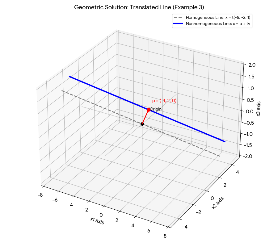
Notice that \(\vec{v}\) satisfies \(A\vec{x}=\vec{0}\) in Example 1, and \(\vec{p}\) satisfies \(A\vec{x}=\vec{b}\).
Description: The solution set is a line through \(\vec{p}\), parallel to the line that is the solution set of the associated homogeneous System \(A\vec{x}=\vec{0}\). This represents a translation of the line.
Theorem
Suppose \(A\vec{x}=\vec{b}\) is consistent for some given \(\vec{b}\), and let \(\vec{p}\) be a solution. Then the solution set of \(A\vec{x}=\vec{b}\) is the set of all vectors of the form:
Where \(\vec{v}_h\) is any solution of the homogeneous equation \(A\vec{x}=\vec{0}\).