This section applies the theory in preceding sections to obtain important theoretical formulas and a geometric interpretation of the determinant.
(I) Cramer's Rule
Let \( A_{n \times n} = \begin{bmatrix} \vec{a}_1 & \dots & \vec{a}_n \end{bmatrix} \). For any \( \vec{b} \in \mathbb{R}^n \), consider the system \( A\vec{x} = \vec{b} \) where \( \vec{x} = \begin{bmatrix} x_1 \\ \vdots \\ x_n \end{bmatrix} \).
Define \( A_i(\vec{b}) \) as the matrix obtained from \( A \) by replacing Column \( i \) by the vector \( \vec{b} \):
Theorem 7: Cramer's Rule
Let \(A\) be an invertible \(n \times n\) matrix. For any \( \vec{b} \) in \( \mathbb{R}^n \), the unique solution \(\vec{x}\) of \( A\vec{x} = \vec{b} \) has entries given by:
Note: Cramer's Rule is needed in a variety of theoretical calculations. For example, it can be used to study how the solution of \( A\vec{x} = \vec{b} \) is affected by changes in the entries of \( \vec{b} \). We can also use Cramer's Rule to derive a formula for \(A^{-1}\). However, the formula is generally inefficient for hand calculations on large systems.
Determine the values of the parameter \( s \) for which the system has a unique solution, and describe the solution.
\[ \begin{cases} 3sx_1 + 5x_2 = 3 \\ 12x_1 + 5sx_2 = 2 \end{cases} \]Solution:
By Theorem 5 in Section 2.2, \( A\vec{x} = \vec{b} \) has a unique solution if \(A\) is invertible, which means \(\det A \neq 0\).
\[ A = \begin{bmatrix} 3s & 5 \\ 12 & 5s \end{bmatrix}, \quad \vec{b} = \begin{bmatrix} 3 \\ 2 \end{bmatrix} \]Find the determinant of \(A\):
\[ \det A = \begin{vmatrix} 3s & 5 \\ 12 & 5s \end{vmatrix} = 15s^2 - 60 = 15(s^2 - 4) = 15(s + 2)(s - 2) \]The system has a unique solution when \( \det A \neq 0 \), meaning \( s \neq \pm 2 \).
Now apply Cramer's Rule to describe the solution:
\[ \det A_1(\vec{b}) = \begin{vmatrix} 3 & 5 \\ 2 & 5s \end{vmatrix} = 15s - 10 = 5(3s - 2) \] \[ \det A_2(\vec{b}) = \begin{vmatrix} 3s & 3 \\ 12 & 2 \end{vmatrix} = 6s - 36 = 6(s - 6) \]Thus, the entries for the solution are:
\[ x_1 = \frac{\det A_1(\vec{b})}{\det A} = \frac{15s - 10}{15(s+2)(s-2)} = \frac{3s - 2}{3(s+2)(s-2)} \] \[ x_2 = \frac{\det A_2(\vec{b})}{\det A} = \frac{6s - 36}{15(s+2)(s-2)} = \frac{2s - 12}{5(s+2)(s-2)} \](II) A Formula for \(A^{-1}\)
Let \( A_{n \times n} = \begin{bmatrix} \vec{a}_1 & \vec{a}_2 & \dots & \vec{a}_n \end{bmatrix} \).
Let its inverse be denoted by columns: \( A^{-1} = \begin{bmatrix} \vec{v}_1 & \vec{v}_2 & \dots & \vec{v}_n \end{bmatrix} \).
Since \( AA^{-1} = I_n \), we have:
\[ A \begin{bmatrix} \vec{v}_1 & \dots & \vec{v}_n \end{bmatrix} = \begin{bmatrix} A\vec{v}_1 & \dots & A\vec{v}_n \end{bmatrix} = \begin{bmatrix} \vec{e}_1 & \dots & \vec{e}_n \end{bmatrix} \]This implies that \( A\vec{v}_j = \vec{e}_j \). The \(j\)-th column of \(A^{-1}\) is a vector that satisfies \( A\vec{x} = \vec{e}_j \).
By Cramer's Rule, the \((i, j)\)-entry of \(A^{-1}\) is \(x_i\), given by:
\[ x_i = \frac{\det A_i(\vec{e}_j)}{\det A} \]Notice that \( A_i(\vec{e}_j) = \begin{bmatrix} \vec{a}_1 & \dots & \vec{e}_j & \dots & \vec{a}_n \end{bmatrix} \), where \(\vec{e}_j\) is in the \(i\)-th column. Expanding the determinant of \( A_i(\vec{e}_j) \) down the \(i\)-th column (where \(\vec{e}_j\) has a 1 in the \(j\)-th row and 0s elsewhere) yields the \((j, i)\)-cofactor of \(A\):
\[ \det A_i(\vec{e}_j) = (-1)^{j+i} \det A_{ji} = C_{ji} \]Therefore, substituting this back gives:
\[ A^{-1} = \frac{1}{\det A} \begin{bmatrix} C_{11} & C_{21} & \dots & C_{n1} \\ C_{12} & C_{22} & \dots & C_{n2} \\ \vdots & \vdots & \ddots & \vdots \\ C_{1n} & C_{2n} & \dots & C_{nn} \end{bmatrix} \]Notice that the cofactors are transposed! Normally we do rows-cols, but here the indices are swapped. This matrix of cofactors is called the adjugate (or adjoint) of \(A\), denoted as \( \text{adj } A \).
Theorem 8 (An Inverse Formula)
Let \(A\) be an invertible \(n \times n\) matrix. Then:
Fact: \( (\text{adj } A)A = (\det A)I_n \)
Find the inverse of the matrix \( A = \begin{bmatrix} 2 & 1 & 3 \\ 1 & -1 & 1 \\ 1 & 4 & -2 \end{bmatrix} \).
Solution: First, compute the nine cofactors:
\[ C_{11} = -2, \quad C_{12} = 3, \quad C_{13} = 5 \] \[ C_{21} = 14, \quad C_{22} = -7, \quad C_{23} = -7 \] \[ C_{31} = 4, \quad C_{32} = 1, \quad C_{33} = -3 \]Construct the adjugate matrix by transposing the matrix of cofactors:
\[ \text{adj } A = \begin{bmatrix} -2 & 14 & 4 \\ 3 & -7 & 1 \\ 5 & -7 & -3 \end{bmatrix} \]We can compute \(\det A\) directly, or use the fact that \( (\text{adj } A)A = (\det A)I_n \):
\[ (\text{adj } A)A = \begin{bmatrix} -2 & 14 & 4 \\ 3 & -7 & 1 \\ 5 & -7 & -3 \end{bmatrix} \begin{bmatrix} 2 & 1 & 3 \\ 1 & -1 & 1 \\ 1 & 4 & -2 \end{bmatrix} = \begin{bmatrix} 14 & 0 & 0 \\ 0 & 14 & 0 \\ 0 & 0 & 14 \end{bmatrix} = 14 I_3 \]So, \(\det A = 14\). Finally, multiply by \( \frac{1}{\det A} \):
\[ A^{-1} = \frac{1}{\det A} \text{adj } A = \frac{1}{14} \begin{bmatrix} -2 & 14 & 4 \\ 3 & -7 & 1 \\ 5 & -7 & -3 \end{bmatrix} = \begin{bmatrix} -1/7 & 1 & 2/7 \\ 3/14 & -1/2 & 1/14 \\ 5/14 & -1/2 & -3/14 \end{bmatrix} \](Reminder: The algorithm introduced in Section 2.2 often gives a better/more efficient way to compute \(A^{-1}\)).
(III) Determinants as Area or Volume
We will revisit the geometric interpretation of determinants. (Recall Example 3 in Section 3.1).
Theorem 9
If \(A\) is a \(2 \times 2\) matrix, the area of the parallelogram determined by the columns of \(A\) is \(|\det A|\).
If \(A\) is a \(3 \times 3\) matrix, the volume of the parallelepiped determined by the columns of \(A\) is \(|\det A|\).
Main idea of the proof for the \(2 \times 2\) case:
This is visually obvious for a diagonal matrix \( A = \begin{bmatrix} a & 0 \\ 0 & d \end{bmatrix} \) where the area is simply base \(\times\) height (\(|a| \cdot |d|\)). For a general matrix \( A = \begin{bmatrix} \vec{a}_1 & \vec{a}_2 \end{bmatrix} \), it can be transformed into a diagonal matrix using row operations in a way that changes neither the area of the associated parallelogram nor \(|\det A|\).
Calculate the area of the parallelogram determined by the points.
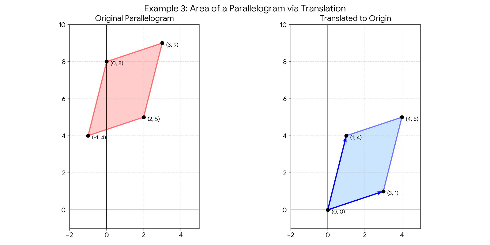
Solution: First, translate the parallelogram to one having the origin as a vertex. Subtract the base vertex from all other vertices. This yields standard vectors radiating from the origin.
Let the translated vectors forming the sides of the parallelogram be \( \begin{bmatrix} 2 \\ -1 \end{bmatrix} \) and \( \begin{bmatrix} 4 \\ 4 \end{bmatrix} \).
Construct the matrix \(A\):
\[ A = \begin{bmatrix} 2 & 4 \\ -1 & 4 \end{bmatrix} \]Find the determinant:
\[ |\det A| = |(2)(4) - (-1)(4)| = |8 + 4| = 12 \]The area of the parallelogram is \( 12 \).
(IV) Linear Transformations
Theorem 10
Let \(T: \mathbb{R}^2 \rightarrow \mathbb{R}^2\) be the linear transformation determined by a \(2 \times 2\) matrix \(A\). If \(S\) is a parallelogram in \(\mathbb{R}^2\), then:
If \(T: \mathbb{R}^3 \rightarrow \mathbb{R}^3\) is determined by a \(3 \times 3\) matrix \(A\), and \(S\) is a parallelepiped in \(\mathbb{R}^3\), then:
It holds whenever \(S\) is a region with a finite area / finite volume.
Let \(S\) be the parallelogram determined by \( \vec{b}_1 = \begin{bmatrix} -2 \\ 3 \end{bmatrix} \) and \( \vec{b}_2 = \begin{bmatrix} -2 \\ 5 \end{bmatrix} \), and let \( A = \begin{bmatrix} 6 & -3 \\ -3 & 2 \end{bmatrix} \).
Compute the area of the image of \(S\) under the mapping \( \vec{x} \mapsto A\vec{x} \).
Solution:
First, find the area of the original parallelogram \(S\):
\[ \text{Area of } S = \left| \det \begin{bmatrix} -2 & -2 \\ 3 & 5 \end{bmatrix} \right| = |(-2)(5) - (-2)(3)| = |-10 + 6| = |-4| = 4 \]Next, find the determinant of the transformation matrix \(A\):
\[ \det A = (6)(2) - (-3)(-3) = 12 - 9 = 3 \]Apply the theorem to find the area of the transformed region \(T(S)\):
\[ \text{Area of } T(S) = |\det A| \cdot (\text{Area of } S) = 3 \cdot 4 = 12 \]