Recall from Section 1.9 that any linear transformation \(T: \mathbb{R}^n \rightarrow \mathbb{R}^m\) can be implemented via left-multiplication by a matrix \(A\): \(\vec{x} \mapsto A\vec{x}\). \(A\) is called the standard matrix of \(T\). Now we need the same sort of representation for any linear transformation between two finite-dimensional vector spaces.
(I) The Matrix of a Linear Transformation
Let \(V\) be an \(n\)-dimensional vector space with basis \(\mathcal{B} = \{\vec{b}_1, \dots, \vec{b}_n\}\).
Let \(W\) be an \(m\)-dimensional vector space with basis \(\mathcal{C} = \{\vec{c}_1, \dots, \vec{c}_m\}\).
Recall from Section 2.9 and 4.4 that the coordinate mapping is a one-to-one linear transformation:
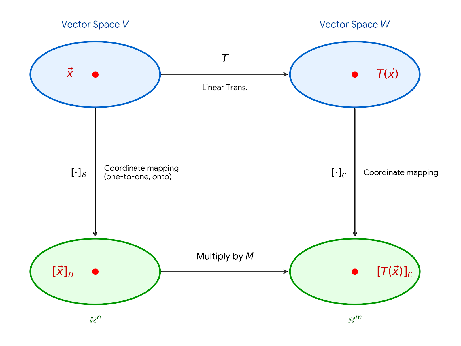
For a linear transformation \(T\), we want to find the connection between \([\vec{x}]_{\mathcal{B}}\) and \([T(\vec{x})]_{\mathcal{C}}\).
If \(\vec{x} = r_1\vec{b}_1 + \dots + r_n\vec{b}_n\), then \([\vec{x}]_{\mathcal{B}} = \begin{bmatrix} r_1 \\ \vdots \\ r_n \end{bmatrix}. \)
Since T is linear,
\( T(\vec{x}) = T(r_1\vec{b}_1 + \dots + r_n\vec{b}_n) \\ = r_1T(\vec{b}_1) + \dots + r_nT(\vec{b}_n) \)
Since the coordinate mapping is linear, we can write:
\( [T(\vec{x})]_{\mathcal{C}} = r_1[T(\vec{b}_1)]_{\mathcal{C}} + \dots + r_n[T(\vec{b}_n)]_{\mathcal{C}}\)Definition
We can write this relation as:
where \(M\) is a matrix representation of \(T\) called the matrix for \(T\) relative to bases \(\mathcal{B}\) and \(\mathcal{C}\):
Suppose \(\mathcal{B} = \{\vec{b}_1, \vec{b}_2\}\) is a basis for \(V\) and \(\mathcal{C} = \{\vec{c}_1, \vec{c}_2, \vec{c}_3\}\) is a basis for \(W\). Let \(T: V \rightarrow W\) be a linear transformation with the property that:
Find the matrix \(M\) for \(T\) relative to \(\mathcal{B}\) and \(\mathcal{C}\).
Solution: The coordinate vectors are the columns of the matrix \(M\).
Let \(\mathcal{B} = \{\vec{b}_1, \vec{b}_2, \vec{b}_3\}\) be a basis for a vector space \(V\) and \(T: V \rightarrow \mathbb{R}^2\) be a linear transformation with the property that:
\[ T(x_1\vec{b}_1 + x_2\vec{b}_2 + x_3\vec{b}_3) = \begin{bmatrix} 2x_1 - 4x_2 + 5x_3 \\ -x_2 + 3x_3 \end{bmatrix} \]Find the matrix for \(T\) relative to \(\mathcal{B}\) and the standard basis for \(\mathbb{R}^2\).
Solution: Evaluate \(T\) at each basis vector \(\vec{b}_i\):
Since we are using the standard basis \(\mathcal{C} = \left\{ \begin{bmatrix} 1 \\ 0 \end{bmatrix}, \begin{bmatrix} 0 \\ 1 \end{bmatrix} \right\}\), the coordinates are simply the entries of the resulting vectors. Thus:
(II) Linear Transformation from V into V (\(V=W\), \(\mathcal{B}=\mathcal{C}\))
If \(V = W\) and we use the same basis \(\mathcal{B}\) for both the domain and codomain, \(M\) is called the matrix for \(T\) relative to \(\mathcal{B}\), or simply the \(\mathcal{B}\)-matrix for \(T\). It is denoted as \([T]_{\mathcal{B}}\).
where:
The mapping \(T: \mathbb{P}_2 \rightarrow \mathbb{P}_2\) defined by \(T(a_0 + a_1t + a_2t^2) = a_1 + 2a_2t\) is a linear transformation.
(1) Find \([T]_{\mathcal{B}}\), where \(\mathcal{B} = \{1, t, t^2\}\).
Solution: Evaluate \(T\) at each basis vector and express the result as a linear combination of the basis vectors:
Extracting the coordinates into columns, we get:
(2) Verify that \([T(\vec{p})]_{\mathcal{B}} = [T]_{\mathcal{B}}[\vec{p}]_{\mathcal{B}}\) for each \(\vec{p}\) in \(\mathbb{P}_2\).
Solution: For any polynomial \(\vec{p}(t) = a_0 + a_1t + a_2t^2\), its image under \(T\) is \(a_1 + 2a_2t\). Thus, its coordinate vector is:
Both expressions yield the same coordinate vector, verifying the relationship.
The mapping \(T: \mathbb{P}_2 \rightarrow \mathbb{P}_2\) defined by \(T(p(t)) = p(1)t^2 - p(2)t + p(-1)\).
Find the matrix \([T]_{\mathcal{B}}\) for \(T\) relative to \(\mathcal{B} = \{t^2 - 1, t, 1\}\).
Solution: Compute \(T\) for each basis polynomial:
Extracting the coordinate vectors relative to \(\mathcal{B}\) yields the columns of \([T]_{\mathcal{B}}\):
Let \(\mathbb{M}_{2 \times 2}\) be the 4-dimensional vector space of \(2 \times 2\) matrices, and let \(T: \mathbb{M}_{2 \times 2} \rightarrow \mathbb{M}_{2 \times 2}\) be the linear transformation given by \(T(A) = A + A^T\).
Find \([T]_{\mathcal{B}}\) for the standard basis \(\mathcal{B} = \left\{ \begin{bmatrix} 1 & 0 \\ 0 & 0 \end{bmatrix}, \begin{bmatrix} 0 & 1 \\ 0 & 0 \end{bmatrix}, \begin{bmatrix} 0 & 0 \\ 1 & 0 \end{bmatrix}, \begin{bmatrix} 0 & 0 \\ 0 & 1 \end{bmatrix} \right\}\).
Solution: Apply \(T\) to each basis matrix:
Placing these coordinate vectors into columns gives:
(III) Linear Transformation on \(\mathbb{R}^n\)
For a transformation \(T: \mathbb{R}^n \rightarrow \mathbb{R}^n\) defined by \(\vec{x} \mapsto A\vec{x}\):
Let \(\mathcal{B} = \{\vec{b}_1, \dots, \vec{b}_n\}\) be a basis for \(\mathbb{R}^n\). Let \(P = \begin{bmatrix} \vec{b}_1 & \dots & \vec{b}_n \end{bmatrix}\).
Then \(\vec{x} = c_1\vec{b}_1 + \dots + c_n\vec{b}_n\).
The coordinate mapping is \(\mathbb{R}^n \rightarrow \mathbb{R}^n\), mapping \(\vec{x} \mapsto [\vec{x}]_{\mathcal{B}}\).
We know that \(\vec{x} = P[\vec{x}]_{\mathcal{B}}\) and \([\vec{x}]_{\mathcal{B}} = P^{-1}\vec{x}\).
![A commutative diagram illustrating similarity of matrix representations on R^n. The top row features two blue ovals representing R^n in the standard basis, with a bold red point x mapping to a bold red point Ax via a horizontal arrow labeled 'Multiply by A'. The bottom row features two green ovals representing R^n in a different basis B. Vertical downward arrows labeled 'Multiply by P inverse' map the top red points down to their corresponding coordinate vectors [x]_B and [Ax]_B, also marked as red points. A bottom horizontal arrow maps [x]_B to [Ax]_B, labeled 'Multiply by [T]_B ([T]_B = P^-1 A P)', visually demonstrating that computing the transformation in the new basis is equivalent to the transformation in the standard basis.](Sec5.4_RtoR.png)
If \(A\) is diagonalizable, then there is a basis \(\mathcal{B}\) for \(\mathbb{R}^n\) consisting of eigenvectors of \(A\). Theorem 8 shows that, in this case, the \(\mathcal{B}\)-matrix for \(T\) is diagonal. Diagonalizing \(A\) amounts to finding a diagonal matrix representation of \(\vec{x} \mapsto A\vec{x}\).
Theorem 8 (Diagonal Matrix Representation)
Suppose \(A = PDP^{-1}\) where \(D\) is a diagonal \(n \times n\) matrix. If \(\mathcal{B}\) is the basis for \(\mathbb{R}^n\) formed from the columns of \(P\), then \(D\) is the \(\mathcal{B}\)-matrix for the transformation \(\vec{x} \mapsto A\vec{x}\).
Define \(T: \mathbb{R}^2 \rightarrow \mathbb{R}^2\) by \(T(\vec{x}) = A\vec{x}\), where \( A = \begin{bmatrix} 2 & -6 \\ -1 & 3 \end{bmatrix} \).
Find a basis \(\mathcal{B}\) for \(\mathbb{R}^2\) with the property that \([T]_{\mathcal{B}}\) is diagonal.
Solution: Find the eigenvalues and eigenvectors of \(A\).
\[ \det(A - \lambda I) = \begin{vmatrix} 2-\lambda & -6 \\ -1 & 3-\lambda \end{vmatrix} = (2-\lambda)(3-\lambda) - 6 = \lambda^2 - 5\lambda = \lambda(\lambda - 5) = 0 \]The eigenvalues are \(\lambda = 0, 5\).
For \(\lambda = 0\):
\[ A - 0I = \begin{bmatrix} 2 & -6 \\ -1 & 3 \end{bmatrix} \sim \begin{bmatrix} 1 & -3 \\ 0 & 0 \end{bmatrix} \implies \vec{v}_1 = \begin{bmatrix} 3 \\ 1 \end{bmatrix} \]For \(\lambda = 5\):
\[ A - 5I = \begin{bmatrix} -3 & -6 \\ -1 & -2 \end{bmatrix} \sim \begin{bmatrix} 1 & 2 \\ 0 & 0 \end{bmatrix} \implies \vec{v}_2 = \begin{bmatrix} -2 \\ 1 \end{bmatrix} \]Thus, \(A = PDP^{-1}\) where:
\[ P = \begin{bmatrix} 3 & -2 \\ 1 & 1 \end{bmatrix} \quad \text{and} \quad D = \begin{bmatrix} 0 & 0 \\ 0 & 5 \end{bmatrix} \]By Theorem 8, \([T]_{\mathcal{B}} = D\) when \(\mathcal{B} = \left\{ \begin{bmatrix} 3 \\ 1 \end{bmatrix}, \begin{bmatrix} -2 \\ 1 \end{bmatrix} \right\}\).
The mapping \(\vec{x} \mapsto A\vec{x}\) and \(\vec{u} \mapsto D\vec{u}\) describe the same linear transformation relative to different bases.
(IV) Similarity of Matrix Representation
The proof of Theorem 8 didn't use the information that \(D\) was diagonal. Hence, if \(A\) is similar to a matrix \(C\), say \(A = PCP^{-1}\), then \(C\) is the \(\mathcal{B}\)-matrix for the transformation \(\vec{x} \mapsto A\vec{x}\) where \(\mathcal{B}\) is formed from the columns of \(P\).
Conversely, if \(T: \mathbb{R}^n \rightarrow \mathbb{R}^n\) is defined by \(T(\vec{x}) = A\vec{x}\) and if \(\mathcal{B}\) is any basis for \(\mathbb{R}^n\), then the \(\mathcal{B}\)-matrix for \(T\) is similar to \(A\). In fact, if \(P\) is formed by vectors in \(\mathcal{B}\), then the \(\mathcal{B}\)-matrix is \(P^{-1}AP\).
Let \( A = \begin{bmatrix} 4 & -9 \\ 4 & -8 \end{bmatrix} \), \(\vec{b}_1 = \begin{bmatrix} 3 \\ 2 \end{bmatrix}\), and \(\vec{b}_2 = \begin{bmatrix} 2 \\ 1 \end{bmatrix}\).
Find the \(\mathcal{B}\)-matrix of the transformation \(\vec{x} \mapsto A\vec{x}\).
Solution: If \( P = \begin{bmatrix} \vec{b}_1 & \vec{b}_2 \end{bmatrix} = \begin{bmatrix} 3 & 2 \\ 2 & 1 \end{bmatrix} \), then the \(\mathcal{B}\)-matrix is \(P^{-1}AP\).
First, compute \(AP\):
\[ AP = \begin{bmatrix} 4 & -9 \\ 4 & -8 \end{bmatrix} \begin{bmatrix} 3 & 2 \\ 2 & 1 \end{bmatrix} = \begin{bmatrix} -6 & -1 \\ -4 & 0 \end{bmatrix} \]Next, find \(P^{-1}\):
\[ P^{-1} = \frac{1}{(3)(1) - (2)(2)} \begin{bmatrix} 1 & -2 \\ -2 & 3 \end{bmatrix} = -1 \begin{bmatrix} 1 & -2 \\ -2 & 3 \end{bmatrix} = \begin{bmatrix} -1 & 2 \\ 2 & -3 \end{bmatrix} \]Finally, compute \(P^{-1}(AP)\):