Section 5.5 Complex Eigenvalues

The matrix eigenvalue-eigenvector theory already developed for \(\mathbb{R}^n\) applies equally well to \(\mathbb{C}^n\).

(I) Complex Eigenvalues

Definition

A complex scalar \(\lambda\) satisfies \(\det(A - \lambda I) = 0\) if and only if there is a nonzero vector \(\vec{x}\) in \(\mathbb{C}^n\) such that:

A\vec{x} = \lambda\vec{x}

Here, \(\lambda\) is a (complex) eigenvalue and \(\vec{x}\) is a (complex) eigenvector corresponding to \(\lambda\).

Example 1

Let \( A = \begin{bmatrix} 0 & -1 \\ 1 & 0 \end{bmatrix} \). Find the eigenvalues of \(A\) and find a basis for each eigenspace.

Solution: Find the roots of the characteristic equation:

\[ \det(A - \lambda I) = \begin{vmatrix} -\lambda & -1 \\ 1 & -\lambda \end{vmatrix} = \lambda^2 + 1 = 0 \implies \lambda = i, -i \]

For \(\lambda = i\):

\[ A - iI = \begin{bmatrix} -i & -1 \\ 1 & -i \end{bmatrix} \]

Note: Row reduction is unpleasant by hand because of the complex arithmetic. Since \(i\) is an eigenvalue, the system should have a nontrivial solution. Therefore, both equations determine the same relation between \(x_1\) and \(x_2\).

\[ \begin{cases} -ix_1 - x_2 = 0 \\ x_1 - ix_2 = 0 \end{cases} \]

From the second equation, \(x_1 = ix_2\). Letting \(x_2\) be free, the general solution is:

\[ \vec{x} = x_2 \begin{bmatrix} i \\ 1 \end{bmatrix} \]

Basis for \(\lambda = i\): \(\left\{ \begin{bmatrix} i \\ 1 \end{bmatrix} \right\}\). ( Another common choice is \(\left\{\begin{bmatrix} -1 \\ i \end{bmatrix}\right\}\) )

For \(\lambda = -i\):

\[ A + iI = \begin{bmatrix} i & -1 \\ 1 & i \end{bmatrix} \implies \begin{cases} ix_1 - x_2 = 0 \\ x_1 + ix_2 = 0 \end{cases} \]

From the second equation, \(x_1 = -ix_2\). Letting \(x_2 = 1\), we get:

Basis for \(\lambda = -i\): \(\left\{ \begin{bmatrix} -i \\ 1 \end{bmatrix} \right\}\).( Another common choice is \(\left\{\begin{bmatrix} 1 \\ i \end{bmatrix}\right\}\) )

Example 2

Let \( A = \begin{bmatrix} 4 & 1 \\ -5 & 2 \end{bmatrix} \). Find the eigenvalues of \(A\) and a basis for each eigenspace.

Solution: Find the characteristic polynomial:

\[ \begin{aligned} \det(A - \lambda I) &= \begin{vmatrix} 4-\lambda & 1 \\ -5 & 2-\lambda \end{vmatrix} \\ &= \lambda^2 - 6\lambda + 13 \\ &= (\lambda - 3)^2 + 4 = 0 \end{aligned} \]

Eigenvalues are \(\lambda_1 = 3 + 2i\) and \(\lambda_2 = 3 - 2i\).

For \(\lambda_1 = 3 + 2i\):

\[ A - \lambda_1 I = \begin{bmatrix} 1 - 2i & 1 \\ -5 & -1 - 2i \end{bmatrix} \]

Using the second row for simplicity: \(-5x_1 - (1+2i)x_2 = 0 \implies -5x_1 = (1+2i)x_2\).

Eigenvector (not unique): \(\vec{v}_1 = \begin{bmatrix} -1 - 2i \\ 5 \end{bmatrix}\).

For \(\lambda_2 = 3 - 2i\):

Notice that \(\lambda_2 = \overline{\lambda_1}\). We can verify the result:

\[ A - \lambda_2 I = \begin{bmatrix} 1 + 2i & 1 \\ -5 & -1 + 2i \end{bmatrix} \implies -5x_1 = (1-2i)x_2 \]

Eigenvector: \(\vec{v}_2 = \begin{bmatrix} -1 + 2i \\ 5 \end{bmatrix}\). Note that \(\vec{v}_2 = \overline{\vec{v}_1}\).

(II) Real and Imaginary Parts of Vectors

For a vector \(\vec{x}\) in \(\mathbb{C}^n\):

\(\overline{\vec{x}}\): Complex conjugate of entries in \(\vec{x}\). (\(\overline{\vec{x}} \in \mathbb{C}^n\)).
\(\text{Re } \vec{x}\): Real part of \(\vec{x}\) formed from the real part of the entries of \(\vec{x}\).
\(\text{Im } \vec{x}\): Imaginary part of \(\vec{x}\) formed from the imaginary part of the entries of \(\vec{x}\).

Example 3

Find \(\text{Re } \vec{x}\), \(\overline{\vec{x}}\), and \(\text{Im } \vec{x}\) for \( \vec{x} = \begin{bmatrix} 3-i \\ i \\ 2+5i \end{bmatrix} \).

Solution: We can decompose \(\vec{x}\) as:

\[ \vec{x} = \begin{bmatrix} 3 \\ 0 \\ 2 \end{bmatrix} + \begin{bmatrix} -1 \\ 1 \\ 5 \end{bmatrix}i \]

Thus, we have:

\[ \text{Re } \vec{x} = \begin{bmatrix} 3 \\ 0 \\ 2 \end{bmatrix}, \quad \text{Im } \vec{x} = \begin{bmatrix} -1 \\ 1 \\ 5 \end{bmatrix}, \quad \overline{\vec{x}} = \begin{bmatrix} 3+i \\ -i \\ 2-5i \end{bmatrix} \]

\(\overline{B}\) denotes the matrix whose entries are the complex conjugates of entries in \(B\). The following properties hold:

\(\overline{r\vec{x}} = \bar{r}\overline{\vec{x}}\)
\(\overline{B\vec{x}} = \overline{B}\overline{\vec{x}}\)
\(\overline{Bc} = \overline{B}\overline{c}\)
\(\overline{rB} = \bar{r}\overline{B}\)

(III) Eigenvalues and Eigenvectors of a Real Matrix that Acts on \(\mathbb{C}^n\)

Fact: When \(A\) is real, its complex eigenvalues occur in conjugate pairs.

Let \(A\) be an \(n \times n\) matrix whose entries are real (\(\overline{A} = A\)).

\[ \overline{A\vec{x}} = \overline{A}\overline{\vec{x}} = A\overline{\vec{x}} \] If \(\lambda\) is an eigenvalue of \(A\) and \(\vec{x}\) is a corresponding eigenvector in \(\mathbb{C}^n\), then: \[ \begin{aligned} A\vec{x} &= \lambda\vec{x} \\ \overline{A\vec{x}} &= \overline{\lambda\vec{x}} \\ A\overline{\vec{x}} &= \overline{\lambda}\overline{\vec{x}} \end{aligned} \] \(\overline{\lambda}\) is also an eigenvalue of \(A\), with a corresponding eigenvector \(\overline{\vec{x}}\). (Revisit Example 2 to see this in action). Recall from Appendix B: For a complex number \(z = a + bi\) represented as \((a, b)\): \[ \begin{aligned} a &= r\cos\varphi \\ b &= r\sin\varphi \\ r &= \sqrt{a^2 + b^2} \\ \tan\varphi &= \frac{b}{a} \quad (\varphi \in (-\pi, \pi]) \end{aligned} \] If \(C = \begin{bmatrix} a & -b \\ b & a \end{bmatrix}\), the eigenvalues are \(\lambda = a \pm bi\). \[ C = \begin{bmatrix} r\cos\varphi & -r\sin\varphi \\ r\sin\varphi & r\cos\varphi \end{bmatrix} = \begin{bmatrix} r & 0 \\ 0 & r \end{bmatrix} \begin{bmatrix} \cos\varphi & -\sin\varphi \\ \sin\varphi & \cos\varphi \end{bmatrix} \] This shows \(C\) is the composition of a scaling matrix with scale factor \(r = \sqrt{a^2 + b^2}\) and a rotation matrix (discussed in Section 1.9). The mapping \(\vec{x} \mapsto C\vec{x}\) is the composition of a rotation and a scaling. Example 4 List the eigenvalues of \(A\). The transformation \(\vec{x} \mapsto A\vec{x}\) is the composition of a rotation and a scaling. Give the angle \(\varphi\) of the rotation and the scale factor \(r\). \[ A = \begin{bmatrix} -2\sqrt{3} & 2 \\ -2 & -2\sqrt{3} \end{bmatrix} \] Solution: The eigenvalues are \(\lambda = a \pm bi = -2\sqrt{3} \pm 2i\). Here, \(a = -2\sqrt{3}\) and \(b = -2\). \[ \begin{aligned} r &= \sqrt{(-2\sqrt{3})^2 + (-2)^2} = \sqrt{12 + 4} = \sqrt{16} = 4 \\ \tan\varphi &= \frac{-2}{-2\sqrt{3}} = \frac{1}{\sqrt{3}} = \frac{\sqrt{3}}{3} \\ \cos\varphi &= \frac{a}{r} = \frac{-2\sqrt{3}}{4} = -\frac{\sqrt{3}}{2} < 0 \\ \sin\varphi &= \frac{b}{r} = \frac{-2}{4} = -\frac{1}{2} < 0 \end{aligned} \] Since both cosine and sine are negative, the angle is in the 3rd quadrant. Thus, \(\varphi = -\frac{5\pi}{6}\). A \(2 \times 2\) matrix with a complex eigenvalue is similar to a rotation-scaling matrix. Theorem 9 Let \(A\) be a real \(2 \times 2\) matrix with a complex eigenvalue \(\lambda = a - bi\) (\(b \neq 0\)) and an associated eigenvector \(\vec{v}\) in \(\mathbb{C}^2\). Then: \[ A = PCP^{-1} \] where \(P = \begin{bmatrix} \text{Re } \vec{v} & \text{Im } \vec{v} \end{bmatrix}\) and \(C = \begin{bmatrix} a & -b \\ b & a \end{bmatrix}\). 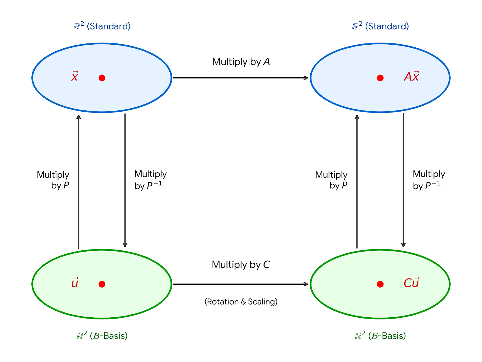Figure: Change of Variable for a Matrix with Complex Eigenvalues (\(A = PCP^{-1}\)) There is a rotation "inside" \(A\). The matrix \(P\) provides a change of variable.