(I) Differential Equations
A linear system of differential equations can be written as:
Here \( x_1, x_2, \dots, x_n \) are differential functions of \( t \) with derivatives \( x_1', x_2', \dots, x_n' \). The coefficients \( a_{ij} \) are constants.
This system can be written in matrix form as:
where \( \vec{x}(t) = \begin{bmatrix} x_1(t) \\ \vdots \\ x_n(t) \end{bmatrix} \), \( \vec{x}'(t) = \begin{bmatrix} x_1'(t) \\ \vdots \\ x_n'(t) \end{bmatrix} \), and \( A = [a_{ij}]_{n \times n} \).
A solution of (1) is a vector-valued function that satisfies (1) for all \( t \) in some interval of real numbers, such as \( t \ge 0 \).
- If both \( \vec{u} \) and \( \vec{v} \) are solutions of \( \vec{x}' = A\vec{x} \), then \( C_1\vec{u} + C_2\vec{v} \) is also a solution. (Property of superposition of solutions)
- The identically zero function is a trivial solution of \( \vec{x}' = A\vec{x} \). Therefore, the set of solutions of \( \vec{x}' = A\vec{x} \) is a subspace of the set of all continuous functions with values in \( \mathbb{R}^n \).
If \( A \) is an \( n \times n \) matrix, then we need to find \( n \) linearly independent solutions of \( \vec{x}' = A\vec{x} \), say \( \vec{x}_1(t), \dots, \vec{x}_n(t) \). These \( n \) functions form a basis of the solution set, and a general solution of (1) is given by:
Initial Value Problem (I.V.P.)
An Initial Value Problem consists of the differential equation and an initial condition:
The unique solution of the I.V.P. is called the particular solution of the I.V.P.
From Calculus, \( \vec{v}e^{\lambda t} \) might be a solution of \( \vec{x}' = A\vec{x} \), where \( \lambda \) is a scalar and \( \vec{v} \) is a nonzero vector.
Let \( \vec{x}(t) = \vec{v}e^{\lambda t} \). Then \( \vec{x}'(t) = \lambda\vec{v}e^{\lambda t} \).
Substitute this into the differential equation \( \vec{x}'(t) = A\vec{x}(t) \):
Since \( e^{\lambda t} \ne 0 \), we can divide by it to obtain:
This shows that \( \lambda \) is an eigenvalue of \( A \) and \( \vec{v} \) is a corresponding eigenvector.
(II) Real Eigenvalues and Graphical Description of Solutions
Consider a \( 2 \times 2 \) matrix \( A \) for the system \( \vec{x}'(t) = A\vec{x}(t) \).
If \( \lambda_1 \) and \( \lambda_2 \) are eigenvalues of \( A \) with associated eigenvectors \( \vec{v}_1 \) and \( \vec{v}_2 \), a general solution is:
The two eigen functions are linearly independent since \( \lambda_1 \ne \lambda_2 \).
A circuit can be described by the differential equation:
where \( x_1 \) and \( x_2 \) are the voltages across the two capacitors at time \( t \).
Suppose \( R_1 = 1 \) ohm, \( R_2 = 2 \) ohm, \( C_1 = 1 \) farad, \( C_2 = 0.5 \) farad. The initial value is \( \vec{x}(0) = \begin{bmatrix} 5 \\ 4 \end{bmatrix} \). Find formulas for \( x_1(t) \) and \( x_2(t) \).
Solution:
Substitute the constants to get the system: \( \vec{x}'(t) = \begin{bmatrix} -1.5 & 0.5 \\ 1 & -1 \end{bmatrix}\vec{x}(t) \) with \( \vec{x}(0) = \begin{bmatrix} 5 \\ 4 \end{bmatrix} \).
The eigenvalues are \( \lambda_1 = -0.5 \) and \( \lambda_2 = -2 \).
For \( \lambda_1 = -0.5 \):
For \( \lambda_2 = -2 \):
A general solution is:
Using the initial condition \( \vec{x}(0) = \begin{bmatrix} 5 \\ 4 \end{bmatrix} \):
The particular solution is:
![A 2D phase portrait illustrating a dynamical system where the origin is an attractor (sink). A solid black line represents the eigenvector v1 = [1, 2], corresponding to the slower decay rate (-0.5). A dashed black line represents the eigenvector v2 = [-1, 1], corresponding to the faster decay rate (-2). Gray stream lines indicate the inward flow of the vector field. Two highlighted trajectories (one in blue starting at (5,4) and one in red starting at (-5,-4)) flow inwards toward the origin. Because the v2 component decays faster, these trajectories swoop inwards and flatten out, approaching the origin tangentially to the solid v1 line, demonstrating the direction of greatest attraction.](Sec5.7Ex1.png)
Graphical Description of Solutions (Phase Portraits)
Case 1: Both eigenvalues are negative.
The origin is an attractor / sink of the dynamical system because all trajectories are drawn into the origin as \( t \to \infty \). The direction of greatest attraction is along the line through the origin and the eigenvector corresponding to the more negative eigenvalue.
Case 2: Both eigenvalues are positive.
The origin is a repeller / source because all trajectories (except the zero solution) turn away from the origin as \( t \to \infty \). The direction of greatest repulsion is the line containing the trajectory of the eigenvector corresponding to the more positive eigenvalue.
Case 3: Eigenvalues have different signs.
The origin is a saddle point. The origin attracts solutions from some directions (along the eigenvector with the negative eigenvalue) and repels them in other directions (along the eigenvector with the positive eigenvalue).
Suppose a particle is moving in a planar force field and its position vector \( \vec{x} \) satisfies \( \vec{x}' = A\vec{x} \), where \( A = \begin{bmatrix} 4 & -5 \\ -2 & 1 \end{bmatrix} \).
Solution: Find the eigenvalues:
The eigenvalues are \( \lambda_1 = 6 \) and \( \lambda_2 = -1 \).
For \( \lambda_1 = 6 \):
For \( \lambda_2 = -1 \):
The general solution is:
Because the eigenvalues have different signs, the origin is a saddle point. Some trajectories approach the origin first and then change direction and move away from the origin.
- The direction of greatest repulsion is the line through \( \vec{v}_1 \) and the origin, corresponding to the positive eigenvalue.
- The direction of greatest attraction is the line through \( \vec{v}_2 \) and the origin, corresponding to the negative eigenvalue.
![A corrected 2D phase portrait illustrating a dynamical system where the origin is a saddle point. A dashed black diagonal line represents the eigenvector v1 = [1, 1], marked with inward arrows indicating attraction due to its negative eigenvalue. A solid black line represents the eigenvector v2 = [-5, 2], marked with outward arrows indicating repulsion due to its positive eigenvalue. Four highlighted trajectories demonstrate the saddle effect: they flow deeply inwards toward the origin parallel to the dashed v1 line, before sharply turning to flow outward indefinitely parallel to the solid v2 line.](Sec5.7Ex2.png)
(III) Complex Eigenvalues
Consider \( \vec{x}' = A\vec{x} \) where \( A \) is a \( 2 \times 2 \) real matrix.
Recall from Section 5.5 that for a real matrix, complex eigenvalues and associated eigenvectors come in conjugate pairs. Suppose \( A \) has a pair of eigenvalues \( \lambda \) and \( \overline{\lambda} \) with associated eigenvectors \( \vec{v} \) and \( \overline{\vec{v}} \).
We have two complex solutions:
A general solution involving complex eigenfunctions is: \( \vec{x}(t) = C_1\vec{v}e^{\lambda t} + C_2\overline{\vec{v}}e^{\overline{\lambda} t} \).
We can extract real solutions using the real and imaginary parts:
A general real solution is:
If \( \lambda = a + bi \), we use Euler's formula:
Solve the I.V.P. \( \vec{x}' = \begin{bmatrix} -5 & 17 \\ -8 & 7 \end{bmatrix}\vec{x} \), with \( \vec{x}(0) = \begin{bmatrix} 4 \\ 2 \end{bmatrix} \).
Solution: Find the eigenvalues:
The eigenvalues are \( \lambda = 1 \pm 10i \).
Choose \( \lambda = 1 + 10i \):
From the second row: \( -8a + (6-10i)b = 0 \implies 4a = (3-5i)b \). Choosing \( b = 4 \), we get \( a = 3-5i \). Thus, \( \vec{v} = \begin{bmatrix} 3-5i \\ 4 \end{bmatrix} \).
Now, compute \( \vec{v}e^{\lambda t} \):
The general real solution is:
Using the initial condition \( \vec{x}(0) = \begin{bmatrix} 4 \\ 2 \end{bmatrix} \):
The particular solution is:
The origin is called a spiral point of the dynamic system. The rotation is caused by the sine and cosine functions. The trajectories spiral outward since \( e^t \to \infty \) as \( t \to \infty \).
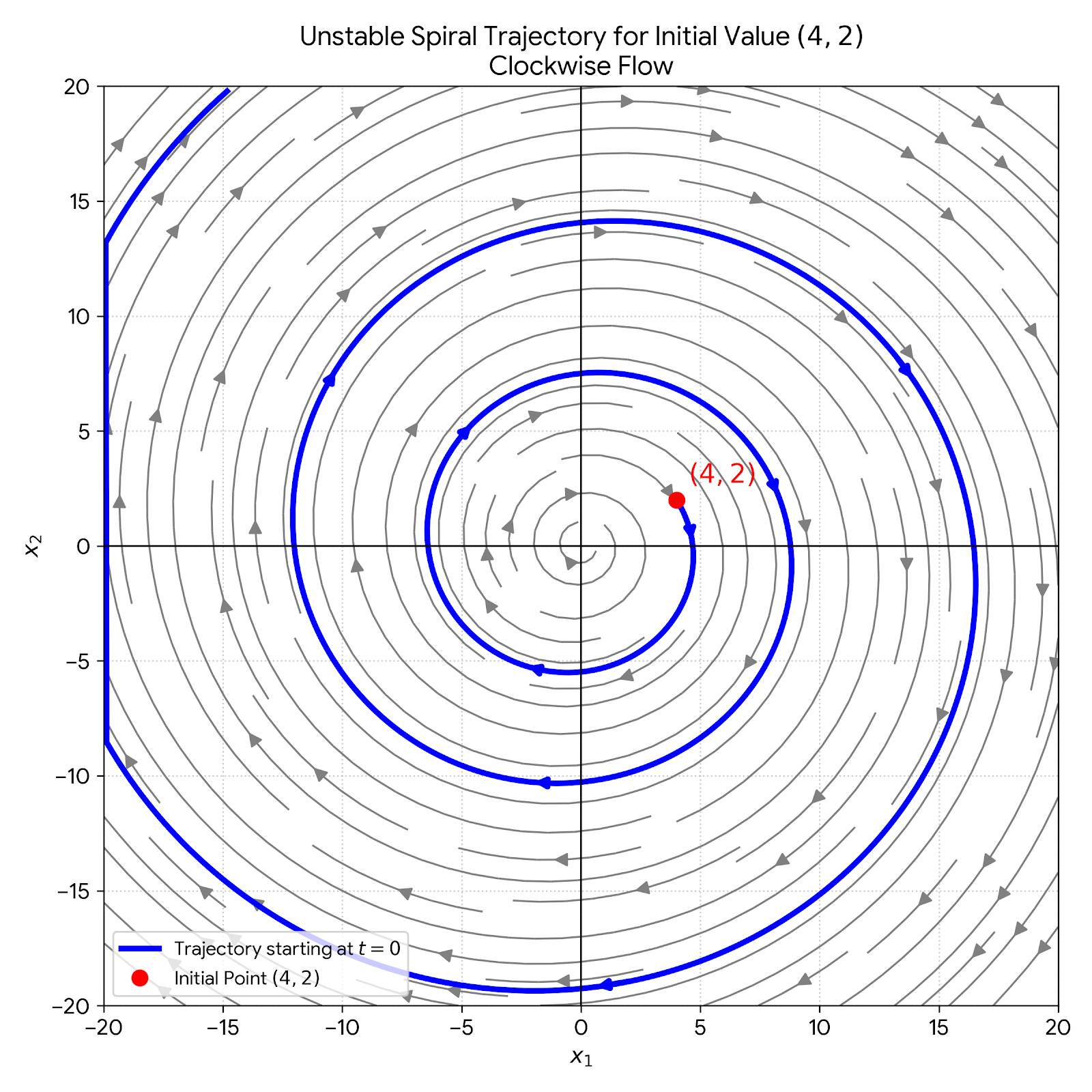
Case 4: Complex Eigenvalues
- If \( A \) has a complex eigenvalue with a positive real part, the trajectories spiral outward. The origin is an unstable spiral.
- If \( A \) has a complex eigenvalue with a negative real part, the trajectories spiral inward. The origin is a stable spiral.
- If \( A \) has a pure imaginary eigenvalue (\( \text{Re } \lambda = 0 \)), the origin is a center. The trajectories are ellipses/circles about the origin.
(IV) Decoupling a Dynamical System
Let \( A \) be an \( n \times n \) diagonalizable matrix with \( n \) linearly independent eigenvectors \( \vec{v}_1, \dots, \vec{v}_n \) corresponding to eigenvalues \( \lambda_1, \dots, \lambda_n \).
Let \( P = \begin{bmatrix} \vec{v}_1 & \dots & \vec{v}_n \end{bmatrix} \) and \( D = \begin{bmatrix} \lambda_1 & \dots & 0 \\ 0 & \dots & \lambda_n \end{bmatrix} \).
For the system \( \vec{x}'(t) = A\vec{x}(t) \), let \( \vec{y}(t) = P^{-1}\vec{x}(t) \), which means \( \vec{x}(t) = P\vec{y}(t) \).
Substitute into the differential equation:
Since \( P \) is invertible, we can left-multiply by \( P^{-1} \) to obtain:
This expands to a system of decoupled equations:
The change of variable from \( \vec{x}(t) \) to \( \vec{y}(t) \) has decoupled the system of differential equations, because the derivative of \( y_k \) depends only on \( y_k \).
The solution for \( \vec{y}(t) \) is:
where \( \vec{y}(0) = \begin{bmatrix} C_1 \\ \vdots \\ C_n \end{bmatrix} = P^{-1}\vec{x}(0) \).
To find the general solution in terms of \( \vec{x} \), multiply back by \( P \):
Make a change of variable that decouples the equation \( \vec{x}' = A\vec{x} \). Write the equation \( \vec{x}(t) = P\vec{y}(t) \) and show the calculation that leads to the uncoupled system \( \vec{y}' = D\vec{y} \), specifying \( P \) and \( D \). Let \( A = \begin{bmatrix} 1 & -2 \\ 3 & -4 \end{bmatrix} \).
Solution: Find the eigenvalues of \( A \):
The eigenvalues are \( \lambda_1 = -2 \) and \( \lambda_2 = -1 \).
For \( \lambda_1 = -2 \):
For \( \lambda_2 = -1 \):
Set \( P \) and \( D \):
Substituting \( \vec{x}(t) = P\vec{y}(t) \) into \( \vec{x}' = A\vec{x} \), we have \( \vec{y}'(t) = D\vec{y}(t) \). That is: