Recall: \( \vec{u} \) and \( \vec{v} \) are orthogonal if \( \vec{u} \cdot \vec{v} = 0 \).
(I) Orthogonal Sets
Definition
A set of vectors \( \{\vec{u}_1, \dots, \vec{u}_p\} \) in \( \mathbb{R}^n \) is said to be an orthogonal set if each pair of distinct vectors from the set is orthogonal. That is, if:
Theorem 4
If \( S = \{\vec{u}_1, \dots, \vec{u}_p\} \) is an orthogonal set of nonzero vectors in \( \mathbb{R}^n \), then \( S \) is linearly independent and hence a basis for the subspace spanned by \( S \).
(Such a set is called an orthogonal basis).
Proof of Theorem 4:
Suppose a linear combination is equal to the zero vector for some scalars \( c_1, \dots, c_p \):
Take the dot product of both sides with \( \vec{u}_1 \):
Since \( \{\vec{u}_1, \dots, \vec{u}_p\} \) is an orthogonal set, \( \vec{u}_j \cdot \vec{u}_1 = 0 \) for \( j = 2, \dots, p \). The equation simplifies to:
Because \( \vec{u}_1 \neq \vec{0} \), we know \( \vec{u}_1 \cdot \vec{u}_1 \neq 0 \). Therefore, \( c_1 = 0 \). By applying the same process with each \( \vec{u}_j \), we find \( c_2 = 0, \dots, c_p = 0 \). Since only the trivial solution exists, the set is linearly independent.
The next theorem suggests why an orthogonal basis is nicer than other bases.
Theorem 5
Let \( \{\vec{u}_1, \dots, \vec{u}_p\} \) be an orthogonal basis for a subspace \( W \) of \( \mathbb{R}^n \). For each \( \vec{y} \) in \( W \):
where the weights are given by:
Proof Idea: To find \( c_j \), compute \( \vec{y} \cdot \vec{u}_j \):
Express \( \vec{y} \) as a linear combination of vectors in \( S \).
Let's denote the vectors in \( S \) as \( \vec{v}_1, \vec{v}_2, \vec{v}_3 \).
Solution:
Old method: Solve the augmented matrix \( [\vec{v}_1 \quad \vec{v}_2 \quad \vec{v}_3 \mid \vec{y}] \).
New method: First, verify \( S \) is an orthogonal set:
So, \( S \) is an orthogonal set and hence an orthogonal basis for \( \mathbb{R}^3 \). By Theorem 5:
Therefore, the decomposition is:
(II) An Orthogonal Projection
Given a nonzero vector \( \vec{u} \) in \( \mathbb{R}^n \), consider decomposing a vector \( \vec{y} \) in \( \mathbb{R}^n \) into the sum:
where \( \vec{z} \) is orthogonal to \( \vec{u} \), and \( \hat{y} \) is a scalar multiple of \( \vec{u} \). Let \( \hat{y} = \alpha\vec{u} \).
Since \( \vec{z} \) is orthogonal to \( \vec{u} \):
Solving for \( \alpha \) gives:
Definition
The orthogonal projection of \( \vec{y} \) onto \( \vec{u} \) is defined as:
If \( L \) is the subspace (line) spanned by \( \vec{u} \), then the projection of \( \vec{y} \) onto \( L \) is denoted \( \text{Proj}_L \vec{y} \). Thus, \( \hat{y} = \text{Proj}_L \vec{y} \).
The distance from \( \vec{y} \) to \( L \) is \( ||\vec{y} - \hat{y}|| = ||\vec{z}|| \).
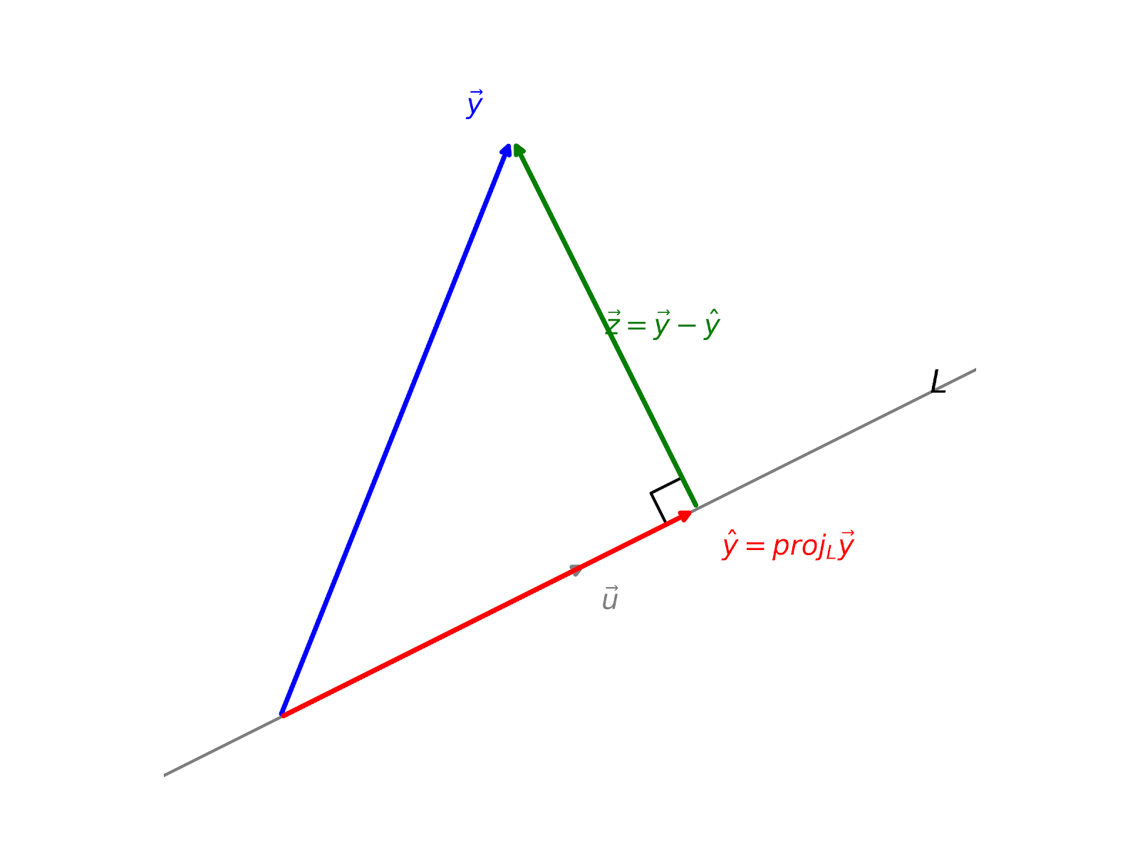
Note: The projection does not change if we scale the vector \( \vec{u} \) by a nonzero scalar \( c \). The projection of \( \vec{y} \) onto \( c\vec{u} \) is:
So, the projection is purely determined by the subspace \( L \) spanned by \( \vec{u} \).
Let \( \vec{y} = \begin{bmatrix} -3 \\ 9 \end{bmatrix} \) and \( \vec{u} = \begin{bmatrix} 1 \\ 2 \end{bmatrix} \). Compute the distance from \( \vec{y} \) to the line through \( \vec{u} \) and the origin.
Solution: First, find the orthogonal projection \( \hat{y} \) of \( \vec{y} \) onto \( \vec{u} \):
The vector representing the distance is \( \vec{z} = \vec{y} - \hat{y} \):
The distance is the length of this vector:
(III) A Geometric Interpretation of Theorem 5
Theorem 5 effectively decomposes a vector \( \vec{y} \) into a sum of orthogonal projections onto one-dimensional subspaces.
For example, if \( W = \mathbb{R}^2 = \text{Span}\{\vec{u}_1, \vec{u}_2\} \) with \( \vec{u}_1 \) and \( \vec{u}_2 \) orthogonal, we can write:
where \( \hat{y}_1 = \text{Proj}_{\vec{u}_1} \vec{y} \) and \( \hat{y}_2 = \text{Proj}_{\vec{u}_2} \vec{y} \).
(IV) Orthonormal Sets
Definition
A set \( \{\vec{u}_1, \dots, \vec{u}_p\} \) is an orthonormal set if it is an orthogonal set of unit vectors (meaning each vector has a length of \( 1 \)).
(1) Find an orthonormal basis of the subspace spanned by the set \( S \) in Example 1.
Solution: We simply normalize each orthogonal vector from Example 1.
(2) Let \( U = \begin{bmatrix} \vec{u}_1 & \vec{u}_2 & \vec{u}_3 \end{bmatrix} \). Compute \( U^T U \).
Solution:
Since the vectors form an orthonormal set, \( \vec{u}_i \cdot \vec{u}_i = 1 \) and \( \vec{u}_i \cdot \vec{u}_j = 0 \) for \( i \neq j \). Thus:
Theorem 6
An \( m \times n \) matrix \( U \) has orthonormal columns if and only if:
Theorem 7
Let \( U \) be an \( m \times n \) matrix with orthonormal columns, and let \( \vec{x} \) and \( \vec{y} \) be in \( \mathbb{R}^n \). Then:
- \( ||U\vec{x}|| = ||\vec{x}|| \)
(\(\vec{x} \rightarrow U\vec{x} \) preserves lengths) - \( (U\vec{x}) \cdot (U\vec{y}) = \vec{x} \cdot \vec{y} \)
- \( (U\vec{x}) \cdot (U\vec{y}) = 0 \) if and only if \( \vec{x} \cdot \vec{y} = 0 \)
(\(\vec{x} \rightarrow U\vec{x} \) preserves orthogonality)
Orthogonal Matrices
If \( U \) is a square matrix with orthonormal columns, then Theorem 6 tells us that \( U^{-1} = U^T \).
Definition: An orthogonal matrix is a square invertible matrix \( U \) such that \( U^{-1} = U^T \).