Recall:
where \( \vec{z} = \vec{y} - \hat{y} \) is orthogonal to \( \vec{u} \), and \( \hat{y} = \text{Proj}_L \vec{y} \).
We now replace the line \( L \) with a \( p \)-dimensional vector space \( W \).
Outline:
- \( \vec{y} - \hat{y} \) is orthogonal to \( W \) and \( ||\vec{y} - \hat{y}|| \) is the distance from \( \vec{y} \) to \( W \).
- \( \hat{y} \) is the unique vector in \( W \) for which \( \vec{y} - \hat{y} \) is orthogonal to \( W \).
- \( \hat{y} \) is the unique vector in \( W \) that is closest to \( \vec{y} \).
(I) Orthogonal Projections
Let \( \{\vec{u}_1, \dots, \vec{u}_n\} \) be a basis for \( \mathbb{R}^n \).
Write \( \vec{y} \) as:
where \( \vec{z}_1 \) is a linear combination of some \( \vec{u}_i \)'s, and \( \vec{z}_2 \) is a linear combination of the other \( \vec{u}_i \)'s.
If \( \{\vec{u}_1, \dots, \vec{u}_n\} \) is an orthogonal basis, then \( \vec{z}_2 \in W^\perp \) if \( \vec{z}_1 \in W \).
Theorem 8 (The Orthogonal Decomposition Theorem)
Let \( W \) be a subspace of \( \mathbb{R}^n \) and let \( \{\vec{u}_1, \dots, \vec{u}_p\} \) be an orthogonal basis of \( W \). Then each \( \vec{y} \) in \( \mathbb{R}^n \) can be written uniquely in the form:
where \( \hat{y} \in W \) and \( \vec{z} \in W^\perp \).
In fact, \( \hat{y} \) is given by:
Proof:
"Existence": Similar to Theorem 5.
"Uniqueness": Assume \( \vec{y} = \hat{y} + \vec{z} = \hat{y}_1 + \vec{z}_1 \). Then:
Since the left side is in \( W \) and the right side is in \( W^\perp \), and \( W \cap W^\perp = \{\vec{0}\} \), they must both equal the zero vector. So, \( \hat{y} - \hat{y}_1 = \vec{0} \) and \( \vec{z}_1 - \vec{z} = \vec{0} \), meaning \( \hat{y} = \hat{y}_1 \) and \( \vec{z} = \vec{z}_1 \).
The uniqueness of the decomposition shows that the orthogonal projection \( \hat{y} \) depends only on \( W \) and not on the particular basis of \( W \).
Equation (1) shows that \( \text{Proj}_W \vec{y} \) is the sum of its projections onto one-dimensional subspaces that are mutually orthogonal.
Let \( \vec{u}_1 = \begin{bmatrix} 2 \\ 5 \\ -1 \end{bmatrix} \), \( \vec{u}_2 = \begin{bmatrix} -2 \\ 1 \\ -1 \end{bmatrix} \), and \( \vec{y} = \begin{bmatrix} 1 \\ 2 \\ 3 \end{bmatrix} \). Let \( W = \text{Span}\{\vec{u}_1, \vec{u}_2\} \).
(1) Write \( \vec{y} \) as the sum of a vector in \( W \) and a vector in \( W^\perp \).
Solution: Observe that \( \vec{u}_1 \cdot \vec{u}_2 = 2(-2) + 5(1) + (-1)(-1) = 0 \), and hence \( \{\vec{u}_1, \vec{u}_2\} \) is an orthogonal basis of \( W \).
Check: \( \hat{y} \cdot \vec{z} = (-2/5)(7/5) + (2)(0) + (1/5)(14/5) = -14/25 + 0 + 14/25 = 0 \).
(II) The Best Approximation Theorem
Theorem 9 (The Best Approximation Theorem)
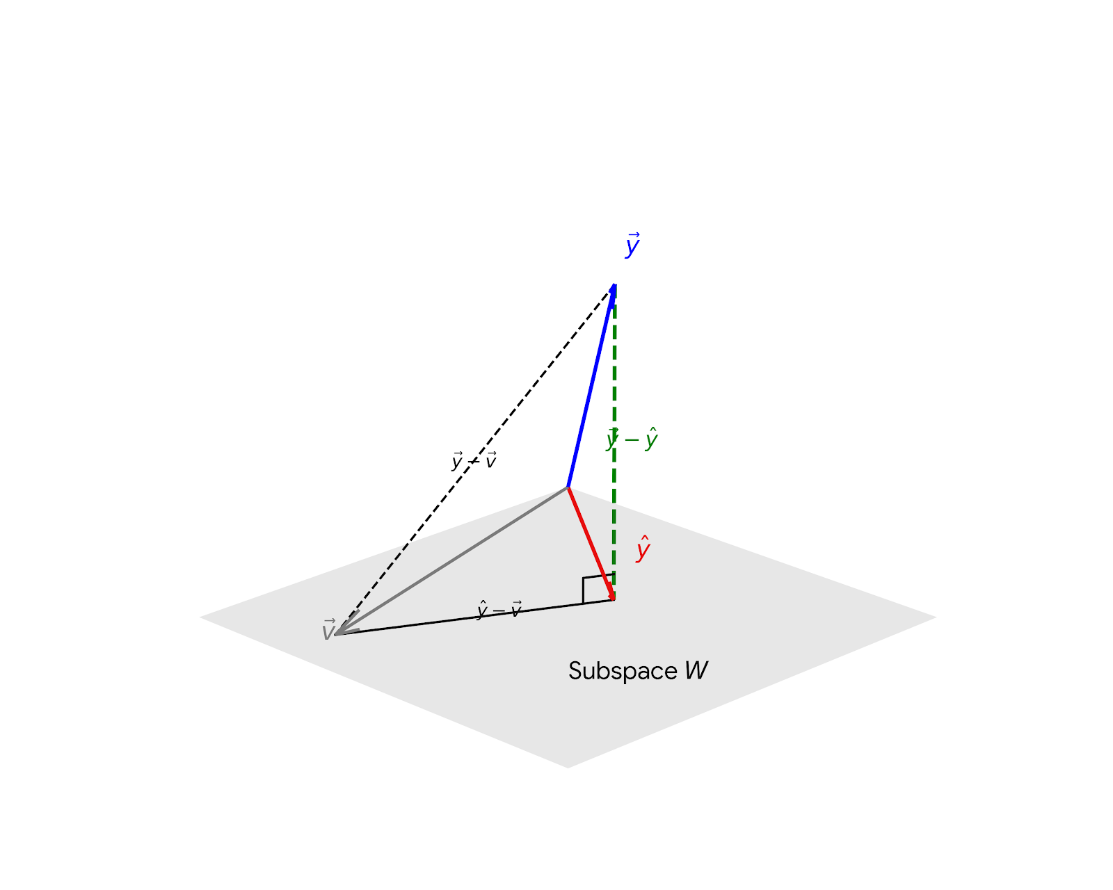
Let \( W \) be a subspace of \( \mathbb{R}^n \). Let \( \vec{y} \) be any vector in \( \mathbb{R}^n \) and let \( \hat{y} = \text{Proj}_W \vec{y} \).
Then \( \hat{y} \) is the closest point in \( W \) to \( \vec{y} \) in the sense that:
for all \( \vec{v} \) in \( W \) distinct from \( \hat{y} \).
Facts:
- \( \vec{y} - \hat{y} \) is in \( W^\perp \implies \vec{y} - \hat{y} \) is perpendicular to \( W \).
- \( ||\vec{y} - \hat{y}|| < ||\vec{y} - \vec{v}|| \) represents the right triangle hypotenuse relationship.
- \( ||\vec{y} - \hat{y}|| \) is the distance from \( \vec{y} \) to \( W \).
- \( \hat{y} \) is the unique closest point in \( W \) to \( \vec{y} \).
- \( \hat{y} \) is the best approximation to \( \vec{y} \) by the elements of \( W \).
- \( ||\vec{y} - \vec{v}|| \) is the "error" of using \( \vec{v} \) in place of \( \vec{y} \).
(2) Find the closest point in \( W \) to \( \vec{y} \).
Solution: The closest point is the projection \( \hat{y} \):
(3) Find the distance from \( \vec{y} \) to \( W \).
Solution: The distance is the length of \( \vec{z} \):
(III) Projections with Orthonormal Bases
The final theorem in this section shows how the formula in Theorem 8 is simplified when the basis for \( W \) is an orthonormal set (meaning \( \vec{u}_i \cdot \vec{u}_i = 1 \) for all \( i \)).
Theorem 10
If \( \{\vec{u}_1, \dots, \vec{u}_p\} \) is an orthonormal basis for a subspace \( W \) of \( \mathbb{R}^n \), then:
If \( U = \begin{bmatrix} \vec{u}_1 & \dots & \vec{u}_p \end{bmatrix} \), then:
for all \( \vec{y} \) in \( \mathbb{R}^n \).
Sketch of Proof:
\( \vec{y} \) is a linear combination of \( \vec{u}_1, \dots, \vec{u}_p \) with weights \( \vec{y} \cdot \vec{u}_1, \dots, \vec{y} \cdot \vec{u}_p \).
Let \( \vec{v}_1 = \begin{bmatrix} 2 \\ 1 \\ 2 \end{bmatrix} \), \( \vec{v}_2 = \begin{bmatrix} -2 \\ 2 \\ 1 \end{bmatrix} \), and \( \vec{v}_3 = \begin{bmatrix} 4 \\ 8 \\ 1 \end{bmatrix} \).
Note that \( \vec{v}_1 \) and \( \vec{v}_2 \) are orthogonal, but \( \vec{v}_3 \) is not orthogonal to \( \vec{v}_1 \) and \( \vec{v}_2 \). It can be shown that \( \vec{v}_3 \) is not in the subspace \( W \) spanned by \( \vec{v}_1 \) and \( \vec{v}_2 \). Use this fact to find a nonzero \( \vec{z} \) in \( \mathbb{R}^3 \) that is orthogonal to \( \vec{v}_1 \) and \( \vec{v}_2 \).
Solution: Apply Theorem 8 with \( \vec{y} = \vec{v}_3 \) and \( W = \text{Span}\{\vec{v}_1, \vec{v}_2\} \).
Find an orthonormal basis \( \{\vec{u}_1, \vec{u}_2\} \) of \( W \) from Example 2 and compute \( U^T U \) and \( U U^T \) for \( U = \begin{bmatrix} \vec{u}_1 & \vec{u}_2 \end{bmatrix} \).
Solution: Normalize \( \vec{v}_1 \) and \( \vec{v}_2 \):
Compute \( U^T U \):
(Matches Theorem 6 in Section 6.2)
Compute \( U U^T \):
Check: We can verify that \( \text{Proj}_W \vec{v}_3 \) (which is \( \hat{v}_3 \) in Example 2) equals \( (U U^T)\vec{v}_3 \).