(I) Introduction
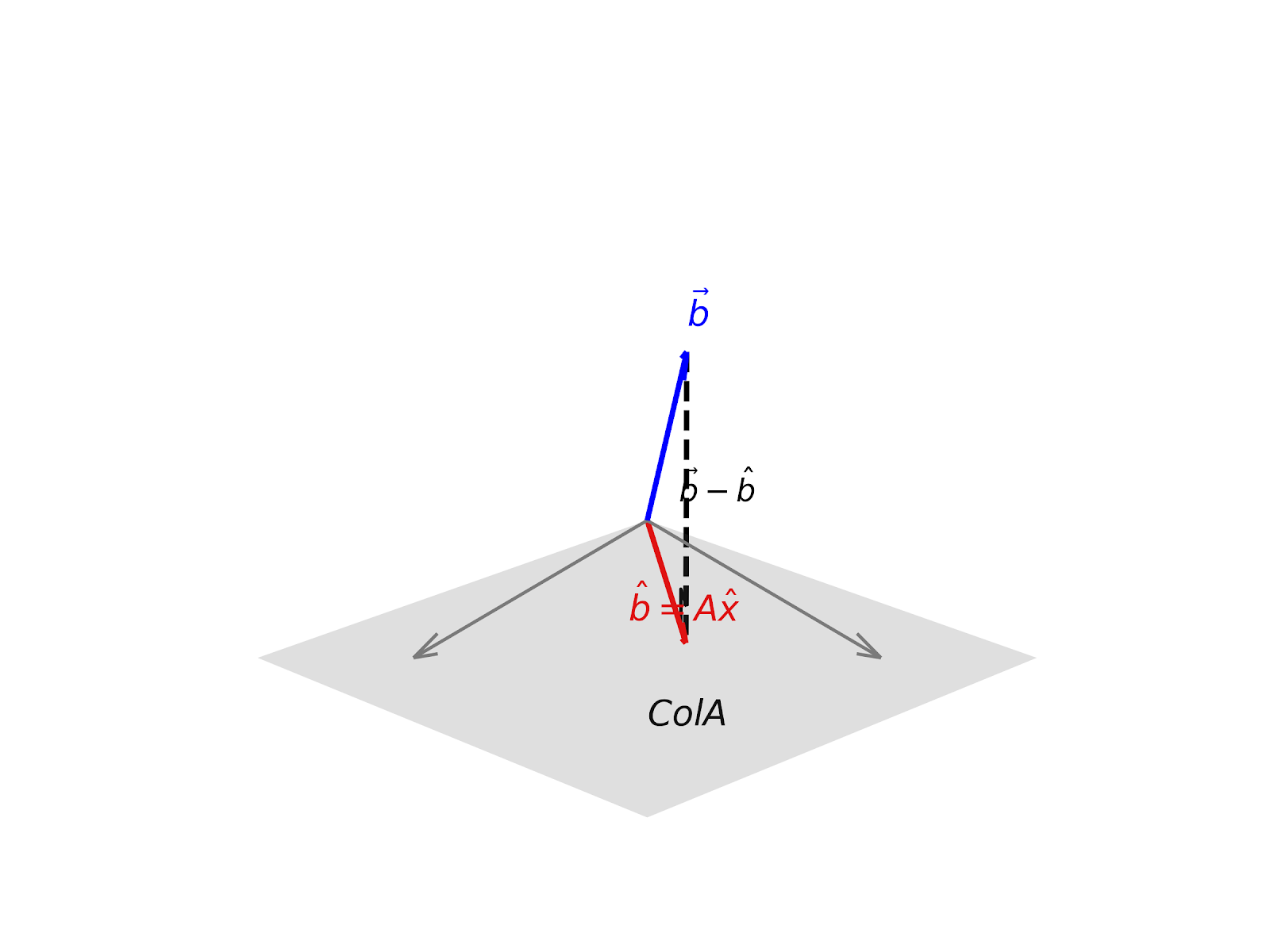
Consider the case when \(A\vec{x} = \vec{b}\) has no solution. When an inconsistent system arises in applications and a solution is demanded, the best one can do is to find an \( \vec{x} \) that makes \( A\vec{x} \) as close as possible to \( \vec{b} \).
Since \( ||\vec{b} - A\vec{x}|| \) is the square root of a sum of squares, the least-squares problem is to find an \( \vec{x} \) that makes \( ||\vec{b} - A\vec{x}|| \) as small as possible.
Definition
If \( A \) is an \( m \times n \) matrix and \( \vec{b} \) is in \( \mathbb{R}^m \), a least-squares solution of \( A\vec{x} = \vec{b} \) is a vector \( \hat{x} \) in \( \mathbb{R}^n \) such that:
\( ||\vec{b} - A\hat{x}|| \) is the least-squares error of approximation.
The set of all the vectors \( A\vec{x} \) is \( \text{Col } A \). \( \hat{b} = \text{Proj}_{\text{Col } A} \vec{b} \) is the closest vector in \( \text{Col } A \) to \( \vec{b} \).
If \( \vec{b} \notin \text{Col } A \), then \( \hat{b} \) is in \( \text{Col } A \), so the system \( A\vec{x} = \hat{b} \) is always consistent.
Conclusion: \( \hat{x} \) is a least-squares solution of \( A\vec{x} = \vec{b} \) if and only if \( \hat{x} \) satisfies \( A\hat{x} = \hat{b} \) (Method 1).
(II) Normal Equations
The orthogonal decomposition theorem (Theorem 8 in Section 6.3) shows that \( \vec{b} - \hat{b} = \vec{b} - A\hat{x} \) is orthogonal to \( \text{Col } A \).
Let \( A = \begin{bmatrix} \vec{a}_1 & \vec{a}_2 & \dots & \vec{a}_n \end{bmatrix} \).
Since \( \vec{b} - A\hat{x} \) is orthogonal to each column of \( A \):
This is equivalent to:
Writing this as a matrix equation gives:
Which simplifies to the normal equation for \( A\vec{x} = \vec{b} \):
Theorem 13
The set of least-squares solutions of \( A\vec{x} = \vec{b} \) coincides with the nonempty set of solutions of the normal equations:
(1) Find a least-squares solution of the inconsistent system for:
Solution: We compute \( A^T A \) and \( A^T\vec{b} \).
Now, solve the augmented matrix for the normal equation \( [A^T A \mid A^T\vec{b}] \):
There is a unique solution: \( \hat{x} = \begin{bmatrix} 1 \\ 1 \end{bmatrix} \).
In fact, if \( A^T A \) is invertible, \( \hat{x} = (A^T A)^{-1}A^T\vec{b} \), and the solution is unique.
(2) Determine the least-squares error in the least-squares solution of \( A\vec{x} = \vec{b} \).
Solution: First compute the estimated vector \( A\hat{x} \):
Now compute the error vector \( \vec{b} - A\hat{x} \):
The least-squares error is the length of this vector:
(III) Criteria for Unique Solution
The next theorem gives useful criteria for determining when there is only one least-squares solution of \( A\vec{x} = \vec{b} \).
Theorem 14
Let \( A \) be an \( m \times n \) matrix. The following statements are logically equivalent:
- The equation \( A\vec{x} = \vec{b} \) has a unique least-squares solution for each \( \vec{b} \) in \( \mathbb{R}^m \).
- The columns of \( A \) are linearly independent.
- The matrix \( A^T A \) is invertible.
When these statements are true, the least-squares solution \( \hat{x} \) is given by:
Note: This formula is mainly for theoretical proofs, not for typical calculations.
#27 Show \( \text{Nul}(A) = \text{Nul}(A^T A) \).
Proof:
Part 1: \( \text{Nul}(A) \subseteq \text{Nul}(A^T A) \)
If \( \vec{x} \in \text{Nul } A \), then \( A\vec{x} = \vec{0} \), and consequently \( A^T A\vec{x} = A^T\vec{0} = \vec{0} \), which implies that \( \vec{x} \in \text{Nul}(A^T A) \).
Part 2: \( \text{Nul}(A^T A) \subseteq \text{Nul}(A) \)
If \( \vec{x} \in \text{Nul}(A^T A) \), then \( A^T A\vec{x} = \vec{0} \). Left multiply by \( \vec{x}^T \):
So, \( \vec{x} \in \text{Nul } A \).
#30 Show \( \text{Rank } A = \text{Rank}(A^T A) \).
Proof:
By the Rank Theorem for the \( m \times n \) matrix \( A \):
By the Rank Theorem for the \( n \times n \) matrix \( A^T A \):
Since \( \text{Nul } A = \text{Nul}(A^T A) \) (from #27), their dimensions are equal, so \( \text{Rank } A = \text{Rank}(A^T A) \).
Proving "b iff c" in Theorem 14:
We know \( \text{Rank } A = n \) if and only if the columns of \( A \) are linearly independent.
Since \( \text{Rank}(A^T A) = \text{Rank } A \), we have \( \text{Rank}(A^T A) = n \) if and only if \( \text{Rank } A = n \), which occurs if and only if the columns of \( A \) are linearly independent.
(IV) Method 1: Using Orthogonal Columns
When the columns of \( A \) are orthogonal, we may use Method 1. We find \( \hat{b} \) directly via orthogonal projection and then solve \( A\hat{x} = \hat{b} \).
Find a least-squares solution of \( A\vec{x} = \vec{b} \) for:
Solution: Note that the columns of \( A \) are orthogonal:
Thus, \( \{\vec{v}_1, \vec{v}_2\} \) is an orthogonal basis for \( \text{Col } A \).
Compute the projection \( \hat{b} = \text{Proj}_{\text{Col } A} \vec{b} \):
Now solve \( A\hat{x} = \hat{b} \):
Since \( \hat{b} = 2\vec{v}_1 + 1\vec{v}_2 \) is already written as a linear combination of the columns of \( A \), the weights are simply the entries of \( \hat{x} \).
Theorem 15
Given an \( m \times n \) matrix \( A \) with linearly independent columns. Let \( A = QR \) be a QR factorization of \( A \) as in Theorem 12 (in Section 6.4).
Then for each \( \vec{b} \) in \( \mathbb{R}^m \), the equation \( A\vec{x} = \vec{b} \) has a unique least-squares solution given by: