Some examples from applications

1. Regression with a convolutional network

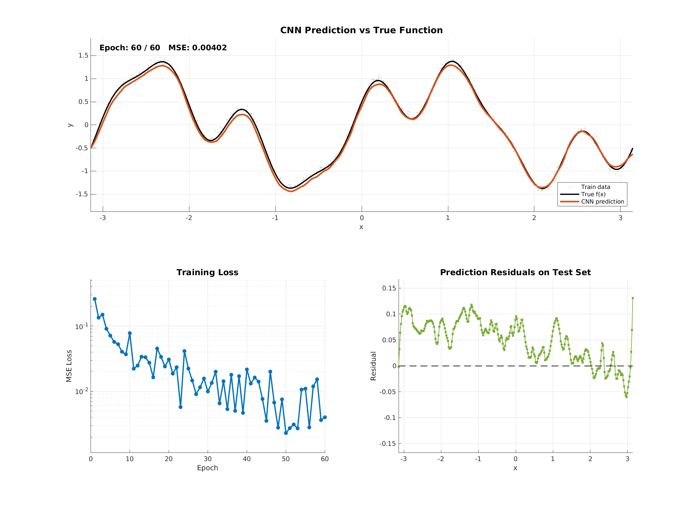
Predicting a continuous output from input features — house prices, molecular binding energies, weather fields. With data $\{(a_i,b_i)\}_{i=1}^n$ and a network $\Phi(\cdot\,;x)$, training minimizes the mean squared error \[ f(x)=\frac1n\sum_{i=1}^n \bigl\|\Phi(a_i;x)-b_i\bigr\|^2. \] With smooth activations (sigmoid, tanh, softplus, GELU), $f$ is a smooth function of the parameters $x$, so this is exactly the setting of Part I.

MATLAB demo: cnn_regression.m — trains a CNN to fit $f(x)=\sin(2x)+0.5\cos(5x)+0.3\sin(8x)$ using Gabor-like patch encoding and the Adam optimizer.

2. Denoising diffusion models

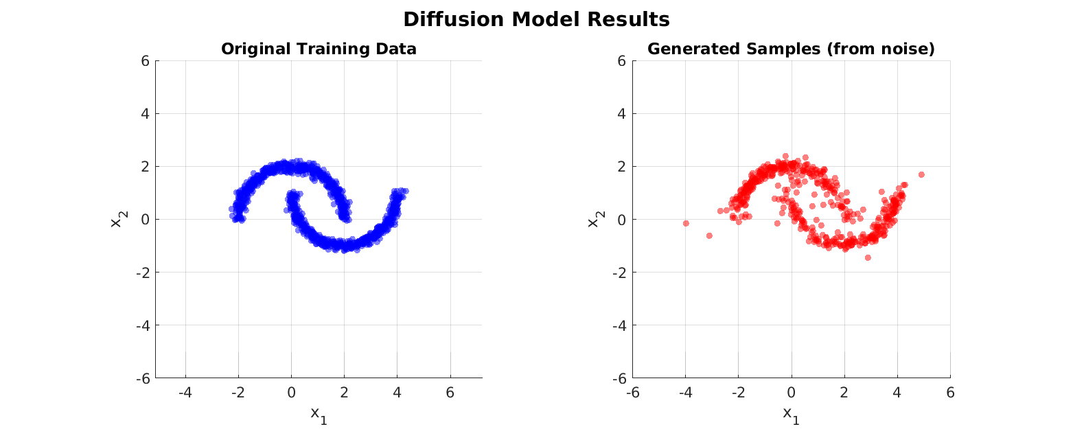
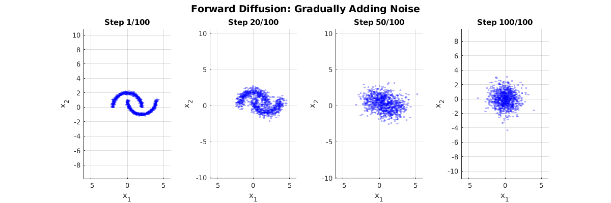
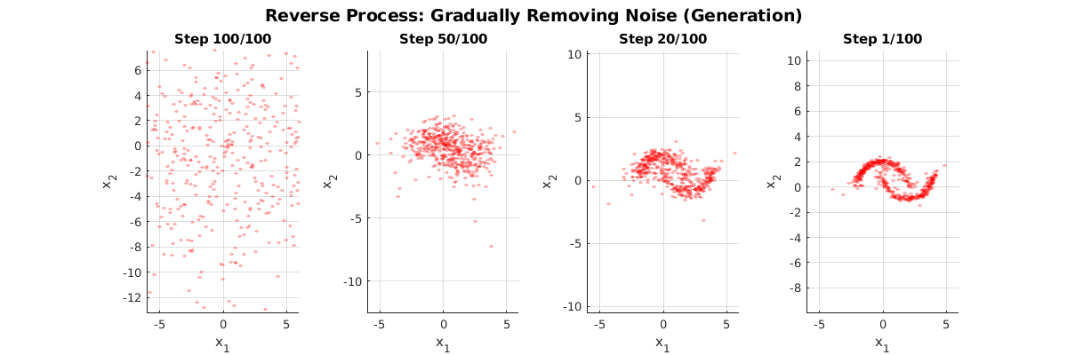
Diffusion models (DDPM, Stable Diffusion, DALL·E 2) generate images by learning to reverse a noise-corruption process. A network $\epsilon_\theta$ is trained to predict the noise added at diffusion step $t$: \[ \mathcal{L}(\theta)=\mathbb{E}_{t,x_0,\epsilon}\bigl[\|\epsilon-\epsilon_\theta(x_t,t)\|^2\bigr], \qquad x_t=\sqrt{\bar\alpha_t}\,x_0+\sqrt{1-\bar\alpha_t}\,\epsilon. \]

Why this is still a smooth problem: smoothness concerns how $\mathcal{L}$ depends on the optimization variable $\theta$, not on the random $(t,x_0,\epsilon)$ or on the sampling procedure used at inference. For each fixed $(t,x_0,\epsilon)$ the integrand is smooth in $\theta$, and the expectation preserves smoothness.

MATLAB demo: diffusion_2d_demo.m — trains a 6-layer fully connected network (512 units, sinusoidal timestep embeddings) on a 2D “two moons” dataset with a cosine noise schedule and a momentum optimizer.

3. Autoencoders

An autoencoder learns a compressed representation by training an encoder–decoder pair to reconstruct its own input: \[ \mathcal{L}(\theta)=\frac1n\sum_{i=1}^n \bigl\|D_\theta(E_\theta(a_i))-a_i\bigr\|^2. \] Applications include dimensionality reduction, denoising, and anomaly detection. Variational autoencoders add a KL-divergence regularizer but keep this MSE reconstruction term.

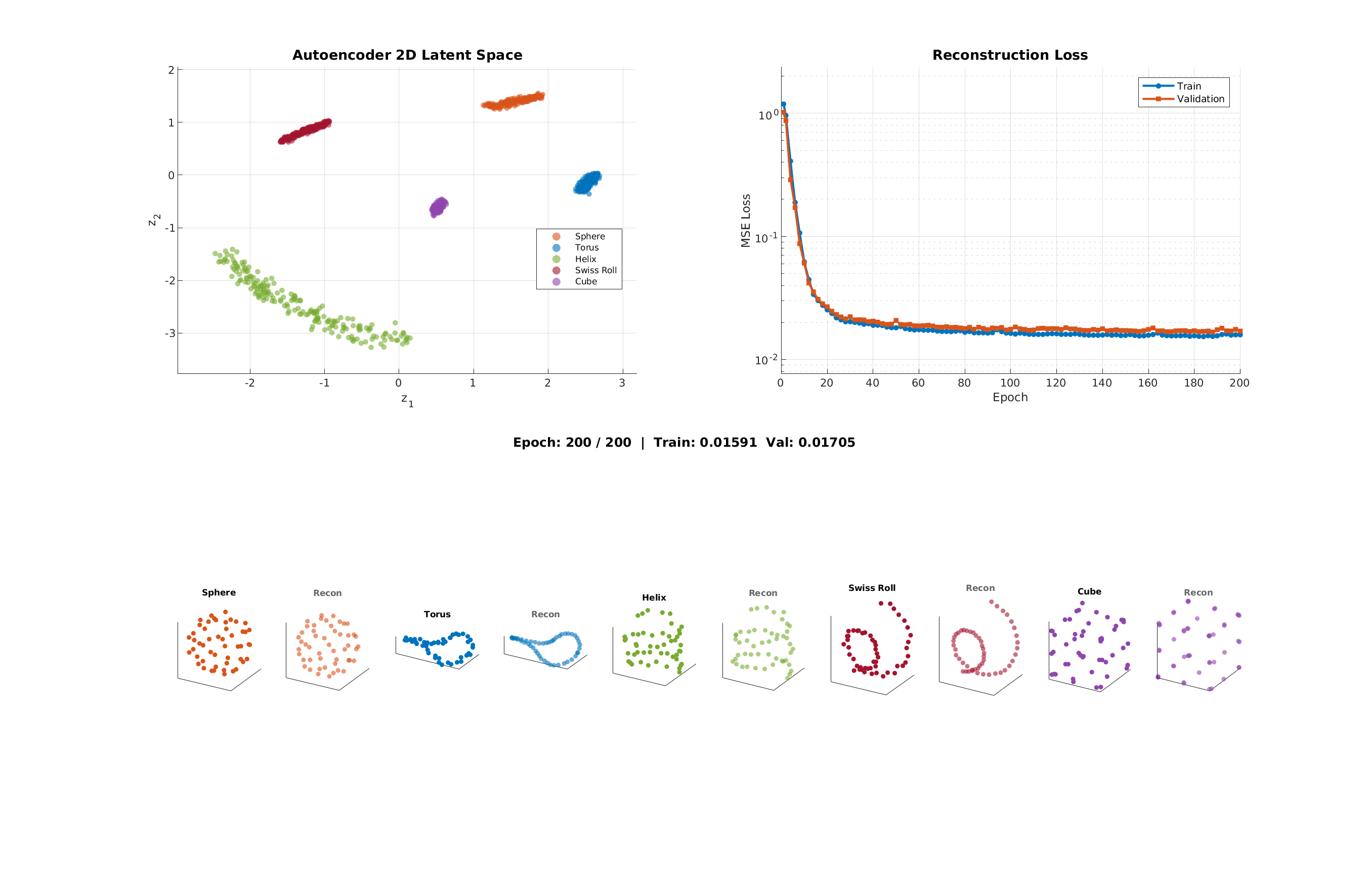
MATLAB demo: autoencoder_pointcloud.m — trains a fully connected autoencoder (150→128→64→32→2→32→64→128→150) that compresses 3D point clouds from 5 shape classes into a 2D latent space.

4. Pretraining a small language model (BERT-Tiny)

Masked language model pretraining is a smooth nonconvex problem: BERT-Tiny uses GELU activations, softmax attention, LayerNorm, and cross-entropy loss, all smooth, so unlike a ReLU network the loss is differentiable everywhere in the parameters.

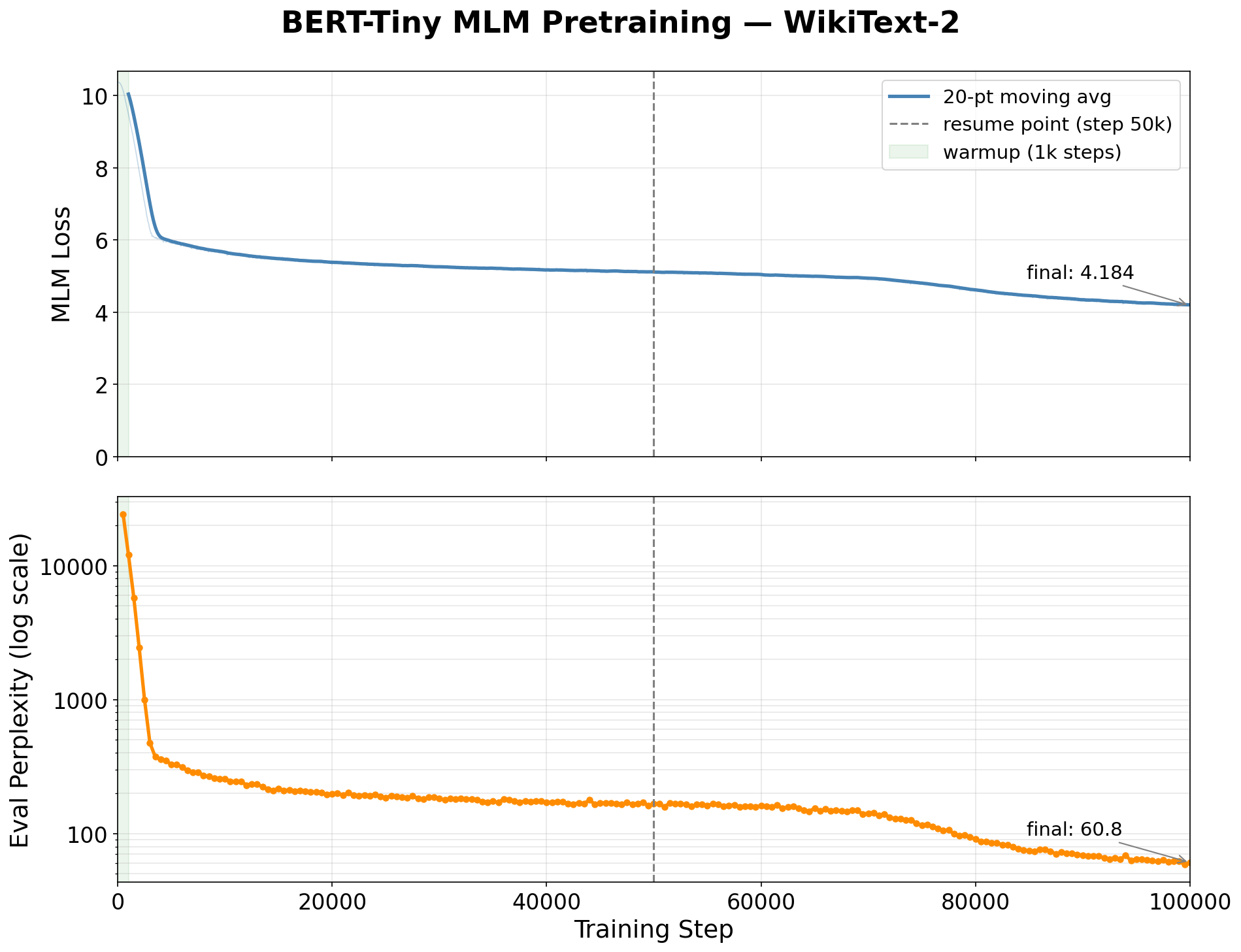
• Architecture: BERT-Tiny, 2 layers, 128 hidden, 2 heads, 4.4M parameters.
• Data: WikiText-2 (~2M tokens), 15% masking; optimizer AdamW, lr $5\times10^{-4}$.
• Training: 100,000 steps, batch size 32. Train loss $10.38 \rightarrow 4.18$; eval perplexity $\approx 24{,}195 \rightarrow 59.4$.

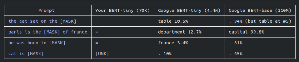
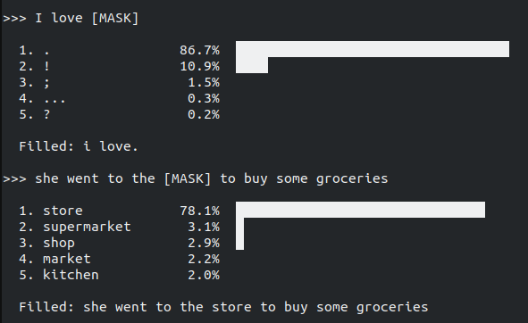
Note that a masked language model is not a chatbot: it fills in blanks, whereas an LLM such as ChatGPT generates text autoregressively and adds instruction tuning and RLHF.

5. Sparse recovery: basis pursuit and the LASSO

Sparse and regularized models (LASSO, elastic net, group LASSO) use $\ell_1$-type penalties, giving nonsmooth convex objectives. The subgradient method applies but is slow, $O(1/\sqrt k)$, and its iterates are not sparse. Exploiting the composite structure $F=f+g$ instead gives the proximal gradient method, where for $g=\lambda\|\cdot\|_1$ the proximal operator is soft-thresholding \[ [\mathrm{prox}_{\alpha\lambda\|\cdot\|_1}(z)]_j=\mathrm{sign}(z_j)\max\bigl(|z_j|-\alpha\lambda,\,0\bigr), \] so every iterate is exactly sparse. The rate is $O(1/k)$ for ISTA and $O(1/k^2)$ for FISTA.

MATLAB demo: douglas_rachford_basis_pursuit.m — solves $\min\|x\|_1$ subject to $Ax=b$ by Douglas–Rachford splitting, alternating affine projection and soft thresholding. It recovers a sparse signal (20 nonzeros in 1000 dimensions) from 100 measurements. For this problem Douglas–Rachford is equivalent to ADMM and to the split Bregman method.

6. Classification with a ReLU network

A ReLU network is a composition of affine maps and the nonsmooth activation $\sigma(t)=\max(t,0)$, which is not differentiable at $t=0$. The training loss is therefore both nonconvex and nonsmooth, and the same is true of networks using max-pooling or dropout. This is the regime that motivates the Clarke subdifferential and the Kurdyka–Łojasiewicz theory.

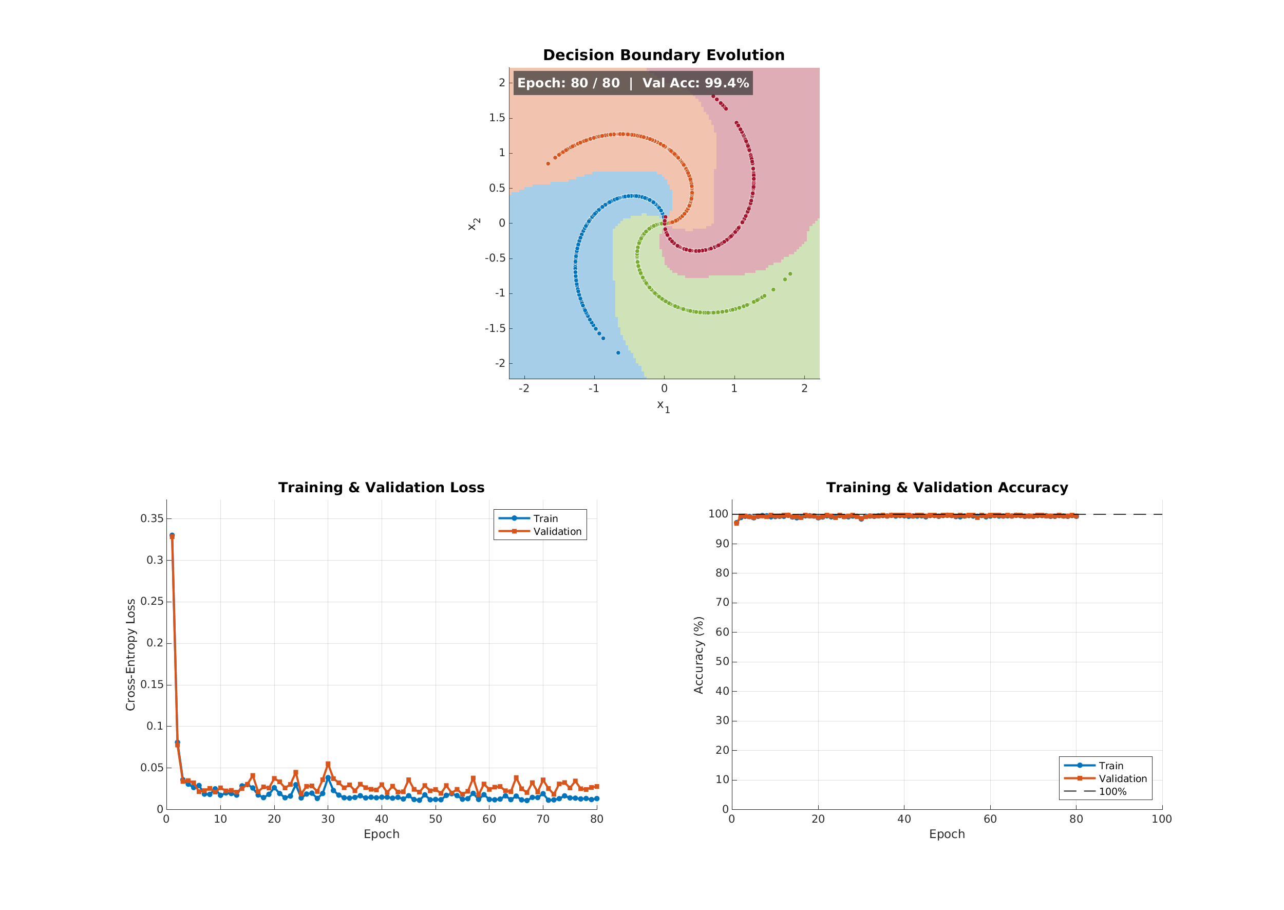
MATLAB demo: cnn_classification.m — trains a CNN to classify a 4-class spiral dataset in 2D using 2D patch encoding, and shows how the decision boundary evolves during training. Concepts: cross-entropy loss, softmax, ReLU, decision boundaries, training/validation split.