MATLAB Educational Demos

Orbital Mechanics

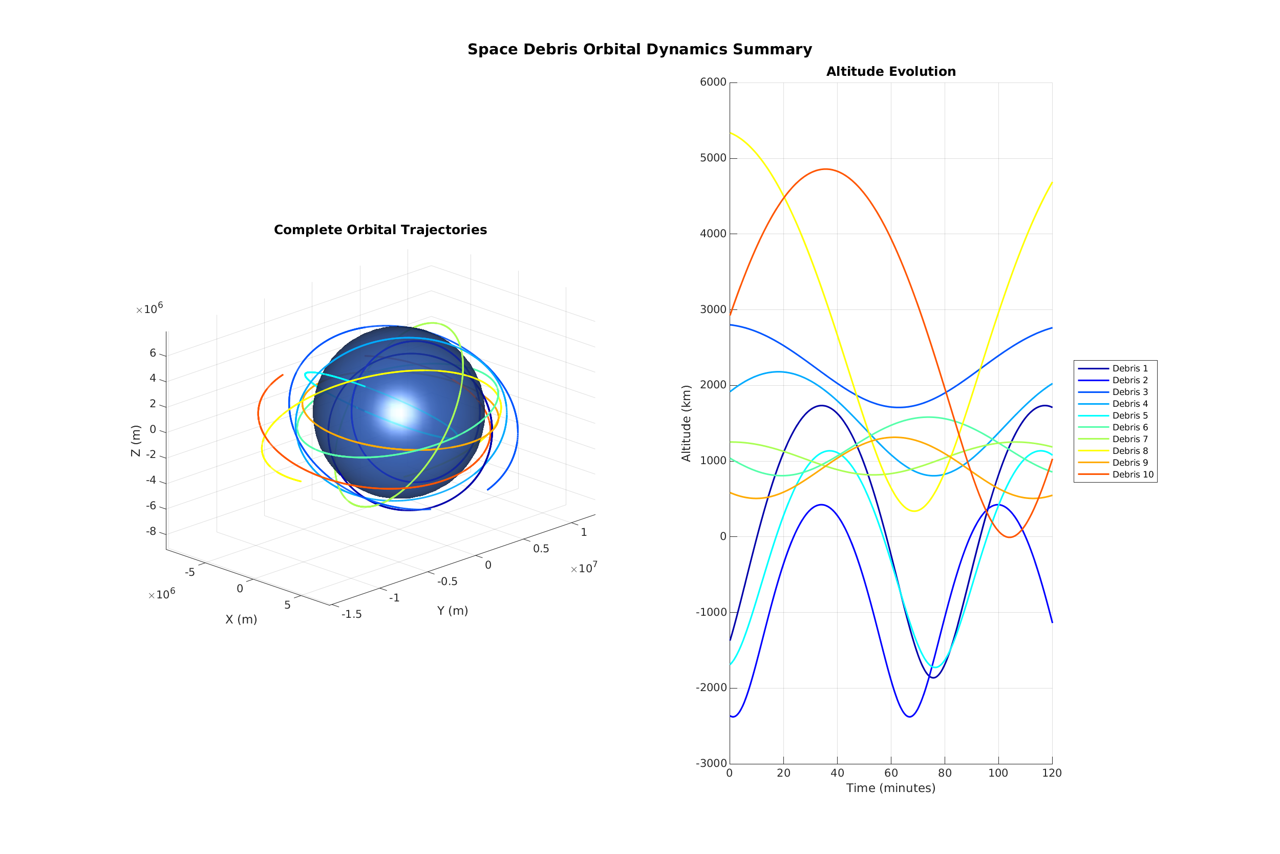
space_debris_simulation.m

Simulates orbital dynamics of 10 debris objects around Earth under gravitational force. Random initial conditions with varying altitudes (300–2000 km), inclinations, and eccentricities.

Method: Numerical integration of Newton's equations in 3D. 2-hour simulation, 10s time step.

Satellite Tracking

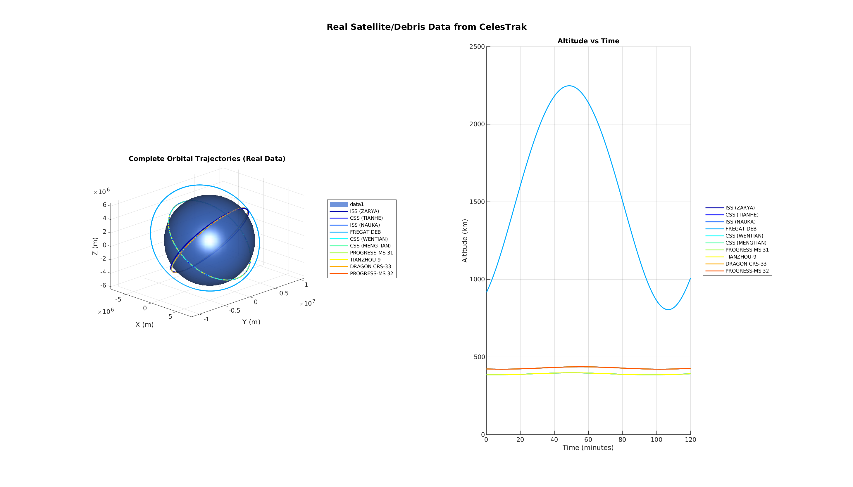
space_debris_real_data.m

Loads real satellite orbital data from TLE (Two-Line Element) format files and propagates orbits using Keplerian elements. 3D visualization of real satellite orbits.

Dataset: iss_tle_data.txt (source: CelesTrak).

Large-Scale Satellites

space_debris_large_dataset.m

Processes and visualizes a large TLE dataset (~14,000+ active satellites). Subsamples 50 for animation and 200 for full trajectory output suitable for operator learning.

Dataset: active_satellites_full.txt (source: CelesTrak active satellites catalog). 2-hour simulation, 15s time step.

Central Limit Theorem

galton_board.m

Simulates balls dropping through a Galton board (peg board) into bins, demonstrating that the resulting distribution approximates a Gaussian. A theoretical normal curve is overlaid on the histogram.

Random Walk (Sphere)

rw_pointcloud.m

Generates 800 uniform points on a unit sphere (Fibonacci spiral), builds a k=10 nearest-neighbor graph, simulates a 5000-step random walk. Stationary distribution is approximately uniform.

Transition rule: Uniform random choice among k nearest neighbors.

Random Walk (Bunny)

rw_bunny.m

Loads Stanford Bunny mesh (8171 vertices), subsamples to 1500 points, builds k=12 nearest-neighbor graph, simulates an 8000-step random walk. Non-uniform density produces a non-uniform stationary distribution.

Dataset: bunny.ply (source: Stanford 3D Scanning Repository).

2D Acoustic Wave Equation

acoustic_wave_2d.m

Simulates wave propagation on a 10×10 m domain with a circular rigid obstacle. A Gaussian pulse is launched from the left side and scatters off the obstacle.

Method: Second-order finite differences in space, leap-frog in time. Dirichlet BCs. 300×300 grid.

Heterogeneous Wave

acoustic_wave_2d_heterogeneous.m

Extends the acoustic wave demo to spatially varying wave speed c(x,y). The medium has horizontal layers, random heterogeneity, and a high-speed lens that focuses waves.

Method: Variable-coefficient wave equation with gradient terms. First-order Mur absorbing BCs. 400×400 grid.

Shock Capturing / CFD

lax_friedrichs_shock_tube.m

Solves the 1D compressible Euler equations for the Lax shock tube problem. Produces a rarefaction wave, contact discontinuity, and shock wave from discontinuous initial data.

Method: First-order Lax-Friedrichs scheme, CFL=0.9. 200 points on [0, 1], final time T=0.14.

Compressed Sensing

douglas_rachford_basis_pursuit.m

Solves basis pursuit (minimize ‖x‖₁ subject to Ax = b) using Douglas-Rachford splitting. Recovers a sparse signal (20 nonzero entries in 1000 dimensions) from 100 measurements.

Method: Douglas-Rachford iteration alternating between affine projection and soft thresholding.

Optimal Transport

optimal_transport_1d.m

Computes and animates optimal transport between two 1D Gaussians using the Benamou-Brenier dynamical formulation. Source: narrow Gaussian at x=−1.5. Target: wider Gaussian at x=1.5.

Method: CDF inversion for the optimal map T(x) = F₁⁻¹(F₀(x)). McCann interpolation for the Wasserstein geodesic.

Optimal Transport (Merge)

optimal_transport_1d_merge.m

Transports a bimodal distribution (two Gaussians at x=−2 and x=2) to a single Gaussian at the origin. Demonstrates how mass from two sources optimally merges into one.

Method: Same CDF-based approach. Animation shows two bumps flowing inward and merging.

MCMC / Langevin Dynamics

langevin_mcmc.m

Demonstrates Langevin dynamics for sampling from a Gibbs distribution using Euler-Maruyama discretization of the Langevin SDE with a double-well potential U(x) = (x²−1)².

Animation: Particle on potential landscape, sample path over time, histogram converging to the Gibbs distribution.

MALA

mala_mcmc.m

Extends Langevin MCMC by adding a Metropolis-Hastings accept/reject step to the Langevin proposal, correcting for discretization bias.

Animation: 4 panels including running acceptance rate plot.

ULA vs MALA Comparison

compare_ula_mala.m

Runs both Unadjusted Langevin (ULA) and MALA side-by-side with the same noise sequence, comparing convergence to the Gibbs distribution via KL divergence.

Animation: Side-by-side histograms, KL divergence on semilogy scale.

CNN Regression

cnn_regression.m

Trains a CNN to fit a smooth function f(x) = sin(2x) + 0.5cos(5x) + 0.3sin(8x). Uses Gabor-like patch encoding to convert 1D input to 2D image patches.

Optimizer: Adam. Animation shows fitted curve evolving during training.

CNN Classification

cnn_classification.m

Trains a CNN to classify a 4-class spiral dataset in 2D. Uses 2D patch encoding and shows decision boundary evolution during training.

Concepts: Cross-entropy loss, softmax, decision boundaries, training/validation split.

Optimizer Comparison

cnn_regression_optimizers.m

Compares 7 optimization methods on the same CNN regression problem: Vanilla GD, SGD, Heavy Ball Momentum, Nesterov, AdaGrad, RMSProp, and Adam. All implemented from scratch with custom training loops.

Animation: 7 fitted curves side-by-side with MSE loss comparison.

Autoencoder

autoencoder_pointcloud.m

Trains an autoencoder (150→128→64→32→2→32→64→128→150) to compress 3D point clouds of 5 shape classes into a 2D latent space. Compares to PCA.

Key insight: Random point ordering makes reconstruction impossible — fixed by deterministic ordered sampling.

AE vs PCA

autoencoder_curved_boundary.m

Designed to show where autoencoders beat PCA. Data lives on a nonlinear manifold (2D latent mapped to 50D via sinusoidal features). Three classes with concentric circular boundaries.

Result: AE achieves ~84% KNN accuracy vs PCA's ~72%.

Diffusion Model

diffusion_2d_demo.m

What are diffusion models? Diffusion models are generative models that learn to create data by learning to reverse a gradual noising process. Imagine a clear photo gradually becoming static over many steps—a diffusion model learns to reverse this, starting from pure noise and gradually removing it to create a clear image.

How they work:

1. Forward Process (Diffusion): Take real data and gradually add Gaussian noise over T timesteps. By the end, data becomes indistinguishable from pure random noise: x₀ → x₁ → ... → xₜ (pure noise).

2. Training: A neural network learns to predict what noise was added at each timestep. Loss = ||ε - ε_θ(xₜ, t)||² (MSE between true and predicted noise).

3. Reverse Process (Generation): Start with pure noise xₜ. The network predicts and removes noise at each step, gradually denoising back to x₀ to generate new samples.

This demo: Uses a 2D "two moons" dataset to visualize the process. 6-layer network (512 units) with sinusoidal timestep embeddings, trained for 5000 epochs with momentum optimizer. Cosine noise schedule with numerical stability fixes.

Key insight: The model successfully generates two crescent shapes from pure noise, though they are noisier and less cleanly separated than the training data. This demonstrates both the power of diffusion models and realistic challenges—sharper, more faithful results would require U-Net architectures with attention, as used in DALL-E and Stable Diffusion.

Visualizations: Forward diffusion | Reverse generation | Final results

Tabular RL

rl_gridworld.m

Solves an 8×8 grid world (obstacles, traps, goal) using exact policy iteration: alternating policy evaluation (Bellman equation) and greedy policy improvement.

Animation: Value function heatmap and policy arrows evolving, then agent following the optimal path.

Deep Q-Network

rl_gridworld_dqn.m

Same grid world, but Q(s,a) is approximated by a neural network (7→64→64→4) trained with Adam and experience replay. Compares learned DQN policy to exact tabular solution.

Result: ~60% policy match vs tabular optimal after 800 episodes.

Mean Field Games

mean_field_game_demo.m

Solves a 1D Mean Field Game for crowd congestion. Agents on [0,1] move toward a target while avoiding congested areas, subject to Brownian noise. The equilibrium balances proximity-to-target against congestion cost.

Method: Fictitious play iterating between HJB backward sweep (Godunov Hamiltonian) and Fokker-Planck forward sweep (upwind advection). Converges in ~27 iterations.

Poisson Convergence

poisson2d_convergence.m

Solves −Δu = f on [0,1]×[0,1] with Dirichlet BCs using second-order finite differences. Manufactured solution u(x,y) = sin(2πx)sin(2πy) provides an exact reference.

Method: 2D Laplacian via Kronecker products. Tests N = 16, 32, 64. Expected: 2nd-order convergence.

Discontinuous Galerkin

dg_euler_2d_positivity.m

Solves the 2D compressible Euler equations using a Q2 Discontinuous Galerkin method with the Zhang-Shu positivity-preserving limiter on a circular explosion benchmark.

Method: Q2 DG, 9 basis functions/element, Gauss-Legendre quadrature. 30×30 elements.

DG Convergence Study

dg_euler_2d_accuracy_test.m

Measures accuracy and convergence rate of the Q2 DG Euler solver using the isentropic vortex benchmark. Tests multiple mesh resolutions and computes L2 errors.

Expected: ~3rd order convergence for Q2 elements on periodic domain.