Now we turn to cubic curves. The study of these was started by Isaac Newton, but the subject didn't really flourish until somewhat later after the advent of complex analysis. Typical cubics are referred to as elliptic curves, which is bit confusing since they are not actually ellipses. The reason for this name comes from its connection to elliptic integrals and functions, where an integral is called elliptic if the integrand contains a square root of cubic polynomial. Below are a few references in addition to the ones given earlier. A classical reference -- in spite of the name -- is Whittaker and Watson [3]. The first two books are more modern.
After adding a point at infinity to the curve on the right, we get two circles topologically. Now let us treat the variables x and y are treated as complex. (In fact, historically signifcant progress in the study of elliptic integrals was made only after the introduction of complex analysis in the 19th century.) Now the above equation defines a complex elliptic curve which topologically is just a torus (after adding a point at infinity). The two real circles are marked in red here and below. We will also keep track of transevrse circle in yellow. It may be helpful to think of this as a "purely imaginary" curve, even though this isn't quite accurate.
The standard way to see this is by using elliptic functions. These are doubly periodic functions with the mildest possible (i.e. inessential) singularities. A function on the complex plane is doubly periodic if its graph repeats itself in both the horizontal and vertical directions. More precisely, we should be able to tile the plane into equally sized parallelograms (called period parallelograms), such that the piece of the graph over each tile is the same. The simplest nonzero example ( in spite of the complicated formula), with period parallelogram having corners at 0, α1,α2 and α1 + α2, is the Weierstrass ℘-function
![∑ [ ]
℘(t) = t-+ -------1-------- -----1------
t2 (m,n)∈Z2-(0,0) (z - m α1 - nα2)2 (m α1 + n α2)2](elliptic_alt6x.png)
 C ,
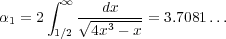
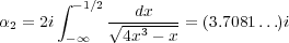
where the periods are expressed by the elliptic integrals
C ,
where the periods are expressed by the elliptic integrals
At this point we can ask whether there exists a rational parameterization of an elliptic curve. The answer is NO. Suppose we could. Then it is possible to show that this extends to a finite to one map of the Riemann sphere (C ∪∞) onto a torus. But this is impossible. The justification of this last statement requires a bit of topology. A version of the Jordan curve theorem says that any closed curve on the sphere would seperate it into two parts (an interior and exterior). If we could find a map as above, we could conclude the Jordan curve holds for the torus: lift the curve up to the sphere and then map the interior/exterior back down. However, it is clear that this isn't true. Just look at the yellow or red curves above.
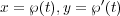
Even though, we now know the elliptic curve abstractly, we really want understand the way it is embedded into C2. As above, we can get a sense of it projecting to 3 real dimensions. The graph of

 ,0,0) ...
is same as in the first example y2 = x.
In particular, the singularities in the graph are artifacts of the projection.
The elliptic curve has none: it's just a torus as we saw. For example, the yellow curve which
is really a loop on the torus gets crushed down to a line in the projection. To get more insight we can
use a different projection. Or better yet, use a family of orthogonal projections:
,0,0) ...
is same as in the first example y2 = x.
In particular, the singularities in the graph are artifacts of the projection.
The elliptic curve has none: it's just a torus as we saw. For example, the yellow curve which
is really a loop on the torus gets crushed down to a line in the projection. To get more insight we can
use a different projection. Or better yet, use a family of orthogonal projections: