A point P
of a curve f(x,y) = 0 is called nonsingular if the gradient ∇f does not vanish at P. In this case, the implicit function
theorem tells us that near P,
y can be
expressed as a function of
x or the other way around.
Most of the curves considered previously (parabola, circle elliptic curve)
consist entirely of nonsingular points. The degenerate conic
consisting of two nonparallel lines has a singularity where they meet.
It is easy to construct singular cubics with several components
as a union of a conic and a line, or three lines.
The nodal cubic
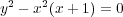 has a singular point at the origin, and it is irreducible
meaning that it is not a union of other curves. From an
algebraic point of view, this amounts to the irreducibility of the
defining polynomial.
The singularity is clearly visible
from the graph over reals. Here we see two tangent directions
at the origin instead of just one.
has a singular point at the origin, and it is irreducible
meaning that it is not a union of other curves. From an
algebraic point of view, this amounts to the irreducibility of the
defining polynomial.
The singularity is clearly visible
from the graph over reals. Here we see two tangent directions
at the origin instead of just one.
In order to plot the complex graph, we reparameterize it by blowing
up the singularity. This means that we seperate the lines at the origin, by
introducing a new variable t = y∕x representing the slope of each line. Plotting this
in x,y,z space, with x = t , yields the so called resolution
of singularities (in black) of the original curve (in red).
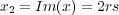
We can find an explicit parameterization by substituting y = xt into
which yields
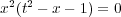 This has two components corresponding to the factorization. These are given by
 depicted in green, and
 in
black. The first two equations give a rational parameterization of the
the original curve.
As we saw the elliptic curve considered above cannot admit such a parametrization.
Thus inspite of the singularity, the present example is simpler.
Setting t = r + is, with r and t real variables, and letting
in
black. The first two equations give a rational parameterization of the
the original curve.
As we saw the elliptic curve considered above cannot admit such a parametrization.
Thus inspite of the singularity, the present example is simpler.
Setting t = r + is, with r and t real variables, and letting
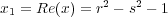
 and
encoding Im(y) as the colour leads to
and
encoding Im(y) as the colour leads to
 Click on picture to start animation.
The real curve is marked in red.
Notice that the graph looks similar to the graph of the
elliptic curve
above. This is because the nodal cubic can be viewed as limit of elliptic
curves
Click on picture to start animation.
The real curve is marked in red.
Notice that the graph looks similar to the graph of the
elliptic curve
above. This is because the nodal cubic can be viewed as limit of elliptic
curves
 as
ε → 0.
In the process, the yellow curve in the previous graph -- called a vanishing cycle in this
context -- shrinks to a point. So the global topology is different; it's no longer a torus. In fact, it's not difficult to see
from the above parameterization that after adding a point at infinity,
we get a sphere with the two points, t = 1 and t = -1, pinched together.
as
ε → 0.
In the process, the yellow curve in the previous graph -- called a vanishing cycle in this
context -- shrinks to a point. So the global topology is different; it's no longer a torus. In fact, it's not difficult to see
from the above parameterization that after adding a point at infinity,
we get a sphere with the two points, t = 1 and t = -1, pinched together.
We next look at another singular example called a (higher order) cusp y2 = x5. It is easy to see that x = t2, y = t5 gives a rational parameterization. This
can arrived at by carrying out a resolution proceedure as above, but
this time with two blow ups. Switching
to polar coordinates (for purely aesthetic reasons) and taking real and imaginary parts as above, leads
to


 This yields
 Now take a look at the outer edge of this picture. The way it is
drawn, it repeatedly crosses itself. But we know this really
represents a defect of our depiction more than anything else.
To get a better feeling for what this ought to look like, form
the intersection of our cusp with a small
sphere
∣x∣2 + ∣y∣2 = ε 2.
This is called the link of the singularity. The sphere can
be identified with R3 plus a point at infinity,
and the link is a knot in this space. In this case, the link
is a so called (2,5)-torus knot which looks as follows
Now take a look at the outer edge of this picture. The way it is
drawn, it repeatedly crosses itself. But we know this really
represents a defect of our depiction more than anything else.
To get a better feeling for what this ought to look like, form
the intersection of our cusp with a small
sphere
∣x∣2 + ∣y∣2 = ε 2.
This is called the link of the singularity. The sphere can
be identified with R3 plus a point at infinity,
and the link is a knot in this space. In this case, the link
is a so called (2,5)-torus knot which looks as follows
 If we did this for a nonsingular point, we would have gotten an
unknotted circle. So the amount of "knottedness" is really telling us how bad
the singularity is.
If we did this for a nonsingular point, we would have gotten an
unknotted circle. So the amount of "knottedness" is really telling us how bad
the singularity is.
Return to first page.
Go to next page.