NumPy For Linear Algebra and Convolutions

NumPy For Linear Algebra and Convolutions

Video

Motivation

If you made it to graduate school in mathematics, I hope I don't have to convince you of the power of matrices. Multiplication, Inversion, and Decomposition have been - or will be - justified to you in linear algebra courses or computation courses.

Your work will tell you what to do with the Matrices - you just need to know how to get them and where the functions are.

NumPy Matrices

In modern NumPy, matrices are represented by two-dimensional arrays. The functions we are used to performing on matrices are instead stored all over the place; as functions in numpy, numpy.linalg, or - for some of the more esoteric things you might use - in the extension scipy. The linalg the documentation lists many options. If what you want isn't there, it may be in scipy.

Of particular note are:

Operation	Math	Example	Notes
Multiplication	$A \cdot B$	`a@b` or `numpy.linalg.matmul(a,b)`
Transposition	$ A^{\text T}$	`A.T`, `A.transpose()`, or `numpy.transpose(A)`
Determinant	$\begin{vmatrix}A\end{vmatrix}$	`numpy.linalg.det(A)`
Inverse	$ A^{-1} $	`numpy.linalg.inv(A)`
Conjugate	$ \overline A $	`A.conj()`
Matrix Exponentiation (by integers)	$A^n$	`numpy.linalg.matrix_power(a,n)`	Much faster than you would think if you have never done it. Uses adapted number-theory calculation techniques.
Matrix Exponentiation (by Matrices)	$e^A$	`scipy.linalg.expm(a)`	If you don't know this, it comes from power series.
Eigenvalues	$\operatorname{Spec}(A)$	`numpy.linalg.eig(a)`	For dimensions greater than 4, uses approximation techniques.
QR Decomposition	$A=QR$	`numpy.linalg.qr(a)`

(almost) all of these are implemented as floating point approximations, as you might have in MatLab. While good enough for most purposes, remember to watch your algorithms for accumulating error, and check your need for a precise value. If you need full precision - and are willing to spend significantly more resources for it - then wait for sympy.

Example: $n$th Fibonacci, but Absurdly Fast

If we represent the Fibonacci numbers as a recurrence matrix, we can calculate the $n$th Fibonacci number incredibly quickly:

import numpy
def fibonacci(n):
    if n<2: return n
    recurrence = numpy.array([[1,1],[1,0]],dtype=numpy.uint64)
    return numpy.linalg.matrix_power(recurrence,n-2)[0].sum()
fibonacci(93)

Though we start running into the limitations of NumPy: as the Fibonacci numbers are exponential, their growth quickly outpaces the size of our integers.

We could approximate the nth value very closely - but for precise calculation, we will see a better way later with sympy.

Advanced Matrix Construction

Slicing

NumPy supports a versatile syntax for slicing - briefly mentioned earlier. Unlike in Python, these don't always create new arrays/lists - but sometimes views, or what is known to linear algebraists as submatrices.

This is significantly faster, and allows for a variety of useful tricks, but can surprise you if you are not ready for it.

For example:

a=numpy.ones((4,5),numpy.int8)
b = a[:,2]
print(b)
b *= 2
print(a)
a[[1,3]] *= 3
print(a)
print(b) # [2,6,2,6]

You can slice matrices on conditions matrices as well, as shown earlier, but this does create a copy when assigned to:

a = numpy.arange(10)
b = a[a%3==1]
print(b)
b *= 2
print(a)

So to apply operations to arrays conditionally, you can use numpy.where:

a = numpy.arange(10)
a
a = numpy.where(a%3 == 1,a+1,a)
print(a) # [0,2,2,3,5,5,6,8,8,9]

Some conditional are so common that they have their own methods. For example, clipping the values at a minimum and/or maximum value can be as easy as:

print(numpy.arange(-4,5).clip(-2,3)) # [-2,-2,-2,-1,0,1,2,3,3]

Reshaping

While some functions allow you to specify a shape, many do not.

You may also be reading provided data and having to put it to form.

For that, ndarray objects have the .reshape property.

A great way to explore reshape is to use arange. For example,

numpy.arange(12).reshape((3,4))

Can show you how values are placed into the new shape of 2x2 array.

Values are placed in lexographic order - the first dimension is completely filled before any value in the second is.

This strict, reliable ordering means that reshape is invariant - so long as the data doesn't change, you will get the same result.

assert numpy.all(numpy.arange(12).reshape((3,4)).reshape((2,6)) == numpy.arange(12).reshape((2,6)))

However, operations in between can lead to somewhat surprising - and occasionally useful - results:

print(numpy.arange(12).reshape((3,4)).transpose().reshape((12)))
# [ 0  4  8  1  5  9  2  6 10  3  7 11]

Matrix Operations

Beyond setting submatrices by slice, and by explicit construction at indices, many common mathematical matrix-building techniques are available:

Operation	Math	Example	Notes
Diagonal	$\operatorname{diag}(1,2,3)$	`numpy.diag([1,2,3])`	If called on a matrix, returns the diagonal entries.
Identity	$I$	`numpy.identity(n)`	The $n \times n$ identity matrix.
Matrix Tensor (Kronecker Product)	$A \otimes B $	`numpy.kron(a,b)`	Standard basis is dictionary ordering.
Block	$\begin{bmatrix} A &B \\ C& D\end{bmatrix}$	`numpy.block([[A,B],[C,D]])`
Block Diagonal	$\begin{bmatrix} A && 0 \\ & B \\ 0 && C \end{bmatrix}$	`scipy.linalg.block_diag(A,B,C)`

Convolution of Data

Convolution of Matrices is a highly efficient technique for locally manipulating data.

In loop notation, one dimensional mathematical convolution could be written:

def convolve(array, kernel):
    ks = kernel.shape[0] # shape gives the dimensions of an array, as a tuple
    final_length = array.shape[0] - ks + 1
    return numpy.array([(array[i:i+ks]*kernel).sum() for i in range(final_length)])

a = numpy.arange(5) # [0,1,2,3,4]
b = convolve(a, numpy.array([1,2])) # [1,3,5,7]
b
numpy.array_equal(b, numpy.array([0+2*1,1+2*2,2+2*3,3+2*4]))

Essentially, it takes moving views of the same length as the kernel, and sums up the entrywise product - a linear combination.

Convolution is a bilinear operation - and distributed - so NumPy can very effectively parallelize it, making it much faster than the loop implementation above.

Convolutions can do a lot of useful computations. With convolutions, you can take rolling averages:

data = [1,2,10,5,4,3]
rolling_average_width = 3
numpy.convolve(data,numpy.ones((rolling_average_width)),mode="valid")

or get the day-by-day change:

numpy.convolve(data,numpy.array([1,-1]),mode="valid")

Or any number of useful rolling linear combinations of your data.

Note the mode="valid". There are three modes in the numpy version - valid is the matrix convolution we know and love from mathematics, which in this case is a little slimmer than the input array.

Higher-Dimensional Convolution

The convolution of higher dimensional NumPy arrays can be achieved with the scipy.signal.convolve or scipy.ndimage.convolve functions - depending on your desired edge behavior mode. (No, I don't know why we can't have just one convolution with all the modes and functionality - but that is how things are.)

You can imagine 2-dimensional convolution as a 1d convolution of convolutions on each axis:

def convolve_1d(array, kernel):
    ks = kernel.shape[0] # shape gives the dimensions of an array, as a tuple
    final_length = array.shape[0] - ks + 1
    return numpy.array([(array[i:i+ks]*kernel).sum() for i in range(final_length)])

def convolve_2d(array,kernel):
  ks = kernel.shape[1] # shape gives the dimensions of an array, as a tuple
  final_height = array.shape[1] - ks + 1
  return numpy.array([convolve_1d(array[:,i:i+ks],kernel) for i in range(final_height)]).T

a = numpy.arange(9).reshape((3,3))
b = numpy.ones((2,2))
c = convolve_2d(a,b)
import scipy.signal
numpy.array_equal(c, scipy.signal.convolve(a,b, mode="valid"))

For a classic example, consider Conway's Game Of Life, in which we have an array of cells. Each cell's behavior at each step depends on the adjacent cells' values in the previous step.

The rules, per Wikipedia at time of writing, are:

Any live cell with fewer than two live neighbours dies, as if by underpopulation.

Any live cell with two or three live neighbours lives on to the next generation.

Any live cell with more than three live neighbours dies, as if by overpopulation.

Any dead cell with exactly three live neighbours becomes a live cell, as if by reproduction.

In this case, the game's rules depend on the sum of the neighbors, and the current binary value.

What Conway stumbled upon is a kind of Matrix Convolution (with a threshold) - in which a value is updated by a linear function on its neighbors.

Convolution of matrices takes a matrix and splits it up into matrix slices centered around each point; in the 3x3 case, reducing it to the data we need to compute the Game of Life.

We then add up a linear function of those entries, represented by the convolution kernel matrix.

We can rewrite Knuth's game of life in NumPy using convolutions:

from scipy.ndimage import convolve
from matplotlib import pyplot
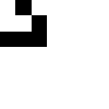
game_board = numpy.zeros((7,7),numpy.int8)
game_board[:3,:3] = [[0,1,0],[0,0,1],[1,1,1]]
pyplot.imshow(game_board,cmap="binary")

neighbor_kernel = numpy.ones((3,3))
neighbor_kernel[1,1] = 0

def life_step(game_board):
    neighbor_sums = convolve(game_board,neighbor_kernel,mode="wrap")

    # If fewer than 2 neighbors, cell is dead.
    game_board[neighbor_sums < 2] = 0
    # If 2 neighbors, cell stays in its state.
    # If 3 neighbors, cell becomes or stays active.
    game_board[neighbor_sums == 3] = 1
    # If >3 neighbors, cell dies
    game_board[neighbor_sums > 3] = 0

life_step(game_board)
pyplot.imshow(game_board,cmap="binary")

Which creates the sequence of images:

Worksheet

Today's worksheet has you creating a couple quick matrices, and practicing a matrix convolution example.