SciKit Learn

Video

Motivation

"Machine Learning" is a buzzword that is big right now, and can mean any number of things - I have seen it used for techniques as basic as linear regression. For many of them, there are several useful tools in Python - such as OpenCV, designed around various image classification, recognition, and processing techniques; or Keras, for so-called Deep Learning - that you can use.

One that has come to my attention recently - though it has been around for a bit over a decade - is SciKit Learn, or sklearn for short. Is focus is on providing a common, abstracted interface to many different machine learning techniques. This can make it fertile ground for people who want to apply math without thinking about the math.

So, over this last weekend, let's go over some of the sklearn tutorial together!

The (supervised) "Machine Learning" Pipeline

Science - that is, formalized learning - has the classic cycle:

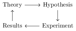
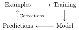
An attempt at formalizing learning for computers has led to a similar supervised learning cycle:

You could spend your entire career studying the methods and tradeoffs in each of these steps and in the movements between them, and people run courses devoted entirely to those tradeoffs. For example, Prof. Buzzard recently ran a course on one family of techniques for this loop, going into a good amount of detail on how it is implemented, why, and in what situations it would be appropriate or how to choose certain parameters.

For a good overview of the basics of machine learning, the Deep Learning textbook chapter goes into considerable depth. I have also seen the O'Reilly Python Data Science Handbook recommended - and while I haven't read it, O'Reilly is a well-established brand in the programming world, and (especially before the modern web) could be found on the shelves of many if not all people who program.

However, most programmers cannot be bothered to learn the mathematics they use, the hows and whys of the models. The software we are using today was - in part - designed for people who want to use these powers without understanding them, and so, we will shy away from the mathematics here.

My hope is that - if this material is of interest to you - the course has prepared you for the programming requirements that most of the Mathematics and Computer Science classes on Machine Learning often list, and you can learn the mathematics in greater detail, over a longer period of time, from people more qualified than I am to speak on it.

SciKit Learn

We have skirted talking about SciPy - and its various SciKits - since we first talked about NumPy.

In general, these are a collection of NumPy-adjacent packages which enable other domains or extensions beyond what NumPy is capable of doing simply on its own; the intentional analogy drawn is with MATLAB Toolboxes.

The one we will be using to day is called scikit-learn, or sklearn for short.

Install it with:

conda install scikit-learn

or

pip install scikit-learn

Depending on platform.

Once it is installed, you can import it:

import sklearn
import numpy

Examples

To learn on some data, we need some data to learn on. For now - while we are following their tutorial - we will be using one of the built-in datasets for this purpose:

from sklearn import datasets
digits = datasets.load_digits()

Data

sklearn's examples store their data in the .data attribute, which we can see is a numpy.ndarray:

type(digits.data)

And if we look at its shape,

digits.data.shape

We can see that it is a 1797x64 2d ndarray.

We can also see what values it takes:

numpy.unique(digits.data)

And it takes the values from 0 to 16 - looks like we have (just over) 4-bit values.

We're expecting a bunch of images, but we got a bunch of 64-length vectors. It's a reasonable guess these are secretly $8 \times 8$ arrays, just reshaped; to find out, let's reshape it back and plot it!

from matplotlib import pyplot
pyplot.imshow(digits.data[0].reshape((8,8)),cmap="Greys")

Well that sure looks like a 0, to us at least!

We can plot another few examples to be sure, but it looks like we have a good representation of the data.

In fact, if we read the documentation for the digits dataset, we can see we are right - and they provide access to these (re)shaped arrays as an ndarray, digits.images.

At this point, we've learned a lot of things about this data - and that sklearn likes its data in 2d form, with rows for each datapoint and columns for the various features of the data.

Target

Supervised Learning - which we are talking about today - deals with examples we already know a lot about. In this case, that knowledge - given by hand-classification of digits - is stored in digits.target as a 1d array:

digits.target.shape
numpy.unique(digits.target)

Looks like these are numpy.int32s, in the range $0-9$.

Models

In Supervised Machine Learning terminology, a Model is your computer's working understanding of the data, which you will Train on examples, and from which you will get Predictions. SciKit learn contains a variety of different kinds of models for different purposes and different technologies, and they provide different interfaces.

The interface we will be looking at today is Estimators.

Estimators

Estimators are constructed a bit differently from eachother, but can provide a common interface. All of them are instances of a class which support a few standard methods - today, we will use .fit, .predict, and .score.

To select one for the job is no easy task - but the SciKit Learn devteam provides a flowchart to help. The tutorial we are following suggests that we use for our first example a Support Vector Machine, and without specialized knowledge, it is worth a try!

The common interface makes it easy to swap it out for another one that might perform better later.

Let's set up our estimator, in this case a svm.SVC.

from sklearn import svm
estimator = svm.SVC(gamma=0.001,C=100.)

The tutorial sets these parameters as black boxes, most likely to avoid overwhelming us. For the mathematically ignorant stumbling in the dark - which, at the moment, likely includes us - the relevant fact is that machine learning systems often contain a variety of arcane parameters, which you can tweak or search to find values that work best without ever understanding why. To help people a bit, the SciKit devs also put up a rough guide for choosing parameters.

Note that, reading the docs, this is just a wrapper around LIBSVM, to bring it to the common interface and make it easy to drop in. This can make it a bit harder to dig into the code - and makes a mathematical understanding even more valuable as a result - but again, we are not doing that today.

Training

Now that we have our estimator, we can use the common interface. Estimators support a fit method:

estimator.fit(digits.data,digits.target)

We can now see it classify an image:

estimator.predict(digits.data[0:10])

But we already told it the answers - that's cheating! (A kind of cheating that has won people many machine learning prizes in competitions, but cheating nonetheless.)

Evaluation

OK, so how do we know it works? We could try it on some unknown data, and check by hand. Or, we could do something a bit cleverer.

People who study Supervised Learning have solved this problem, as they solve many of their problems, with more data.

Instead of training their data on the entire set of known digits, they split it up into 3 parts:

• A Training dataset, on which your model is trained
• A Validation dataset, on which you tweak your model to correct errors
• A Test dataset, on which you check whether your model works on data other than the training data

We don't necessarily know enough now to do Validation, but we can split up our data into a Training and a Test dataset fairly easily with slices or splits:

test_size = 20
test_data,training_data = numpy.split(digits.data,[test_size])
test_target,training_target = numpy.split(digits.target,[test_size])

Note that the size, design, and sampling of these sets is yet another area of academic study, and yet another study I am choosing to ignore today.

Because this is a common task, sklearn provides a utility for doing it (pseudo)randomly:

from sklearn.model_selection import train_test_split
training_data,test_data,training_target,test_target = \
    train_test_split(digits.data,digits.target,test_size=20,random_state=4)

Now we can create a new estimator, free from the bias of the previous training, and see how it does:

estimator = svm.SVC(gamma=0.001,C=100.)
estimator.fit(training_data,training_target)
estimator.predict(test_data) == test_target

The estimators support this kind of testing natively, with another method .score, giving the average:

estimator.score(test_data,test_target)

That's pretty good! It's almost like someone has already chosen an appropriate estimator and parameters for us, to get us excited about Machine Learning in SciKit Learn.

Trying it Out

Creating a New Image

The data - as we've seen - is 8x8 greyscale images. We can make those in Inkscape!

Setup

Open up a new window in Inkscape, and go to the Document Properties. Set the display units to px, and the custom size to 8px by 8px.

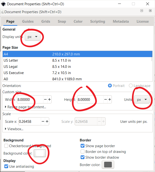
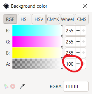
One last thing in this menu - there is no transparency in the example images, so click the background color and slide the "alpha" to 100 - to change from a transparent background to a blank white background.

It may also be nice to set up a 1px by 1px grid, just to see where the pixels are.

When you are done, you may not be able to see your tiny canvas - the View tab is to the rescue here. The View->Zoom->Page - by default, bound to the number 5 - allows you to zoom your page to the window.

Image

In this canvas, select the "Freehand Lines" tool - from the left, or with p - and draw a handwritten digit. Make it large and centered, like in the examples - play around with the Fill & Stroke settings until it looks right. (you should have a line width around 1px).

I drew a 3:

Exporting

Bring up the Export PNG dialog. We want to export the whole Page, and we want to set an Advanced Option; we want to export this as a low-bitdepth Greyscale image. Our target is roughly 4-bits, so we can export it as a Gray_4.

This creates a final PNG:

Classifying our Digit

Loading and Preparing our Image

Now we can load our image:

from matplotlib import image
my_image = image.imread("handdrawn3.png")
pyplot.imshow(my_image,cmap="Greys")

this isn't quite what we had for our classification, so let's coerce it to the values 0-16:

my_image = (16*(1-my_image)).round()
pyplot.imshow(my_image,cmap="Greys")

Applying Our Model

Now let's apply our estimator. It's expecting an array of rows of length $64$, but that's easy to do:

estimator.predict(my_image.reshape((1,64)))

It correctly recognized my hand-drawn 3!

Assignment

Return to the SciKit Learn Estimator Flowchart and follow it, and we will see that it does not recommend SVC for this dataset- instead, it recommends LinearSVC.

Use the last 500 rows as your test data, and the remaining rows as your training data:

training_data,test_data,training_target,test_target = \
    train_test_split(digits.data,digits.target,test_size=500,shuffle=False)

Read the documentation for LinearSVC. Pay particular attention to the parameters - there may be some good advice in the documentation for our particular situation regarding the number of data columns (64) and samples (1297).

Play around with the parameters - especially $C$, which is the main one that can take a variety of values - until your model scores at least 90% on the test data using this new estimator.

Print out this score.

Submit a .py script to Brightspace which creates a LinearSVC which, when trained on the first 1297 rows in the example dataset, scores at least 90% on the last 500. Then the file should train the dataset, and print the score.

You can try out a lot of supervised learning methods, such as sklearn.naive_bayes.GaussianNB, fairly easily using the swappable API.