Skip to main content
Contents Embed Dark Mode Prev Up Next \( \newcommand{\N}{\mathbb N}
\newcommand{\Z}{\mathbb Z}
\newcommand{\Q}{\mathbb Q}
\newcommand{\R}{\mathbb R}
\newcommand{\set}[1]{\{{#1}\}}
\newcommand{\gint}[1]{\llbracket #1 \rrbracket}
\newcommand{\mean}[1]{\overline{#1}}
\newcommand{\median}[1]{\widetilde{#1}}
\newcommand{\spc}[1]{\underline{\hspace{#1}}}
\newcommand{\del}{\partial}
\newcommand{\intfact}{e^{\int P(x) \, dx}}
\newcommand{\defn}{\stackrel{\textrm{def}}{=}}
\newcommand{\laplace}[1]{\mathscr{L}\set{#1}}
\newcommand{\laplaceinv}[1]{\mathscr{L}^{-1}\set{#1}}
\newcommand{\lt}{<}
\newcommand{\gt}{>}
\newcommand{\amp}{&}
\newcommand{\fillinmath}[1]{\mathchoice{\underline{\displaystyle \phantom{\ \,#1\ \,}}}{\underline{\textstyle \phantom{\ \,#1\ \,}}}{\underline{\scriptstyle \phantom{\ \,#1\ \,}}}{\underline{\scriptscriptstyle\phantom{\ \,#1\ \,}}}}
\)
Handout Lesson 10, Equilibrium Solutions and Stability
This lesson is based on Section 2.2 of your textbook by Edwards, Penney, and Calvis.
CITATION: This set of notes contains several slope fields and solution curves sketched in the slope fields. I used the
direction field plotter by Ariel Barton at the Unviersity of Arkansas to create these pictures.
Autonomous Differential Equations, Critical Points, and Equilibrium Solutions.
Definition 62 .
autonomous
\begin{equation*}
\frac{dy}{dx}=f(y)\text{.}
\end{equation*}
Example 63 . Identifying autonomous equations.
\(\frac{dP}{dt}=kP(M-P)\) (This is also a
\(\displaystyle \frac{dy}{dx}=yx^2\)
With the logistic model
\(\frac{dP}{dt}=kP(M-P)$\) \(P \equiv \fillinmath{XXXXXXXXXXXXXXX}\) and
\(P \equiv \fillinmath{XXXXXXXXXXXXXXX}\) are constant solutions. These constant solutions separate the other solutions into three categories, depending on the value of
\(P_0\text{.}\)
Let’s consider the logistic growth model
\begin{equation*}
\frac{dP}{dt}=P(2-P)
\end{equation*}
The following slope field and solution curves were generated by the direction field plotter by Ariel Barton.
A slope field for
\(\frac{dP}{dt}=P(2-P)\text{.}\)
Definition 64 .
The solutions of \(f(y)=0\) are the critical points of the autonomous differential equation
\begin{gather}
\frac{dy}{dx}=f(y)\tag{✶✶}
\end{gather}
If
\(y=c\) is a critical point of
(✶✶) , then the constant solution
\begin{equation*}
y(x)=c \text{ or } y\equiv c
\end{equation*}
is an
equilibrium solution of
(✶✶) .
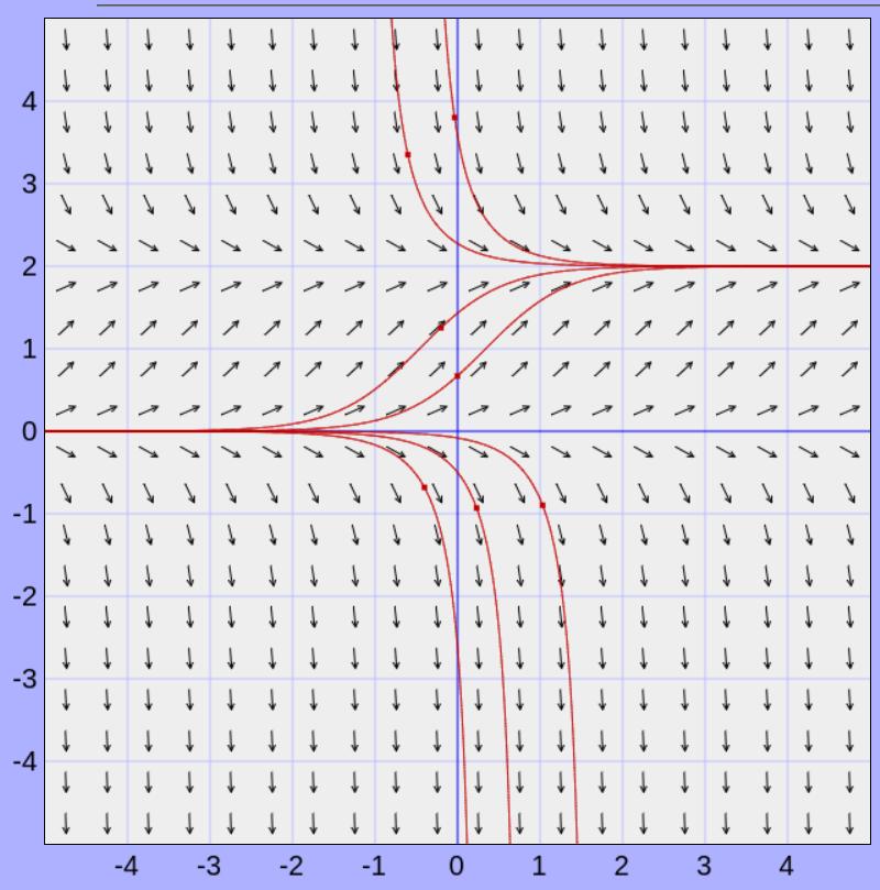
Phase Diagrams and Stability. Let’s take another look at the slope field diagram that we saw earlier for the logistic model
\(\frac{dP}{dt}=P(2-P)\text{.}\)
A slope field for
\(\frac{dP}{dt}=P(2-P)\text{.}\)
As \(t \rightarrow \infty\text{:}\)
the diagram around
\(P \equiv 0\) looks like a “
”. We call
\(P= 0\) an
critical point of the model.
the diagram around $P \equiv M$ looks like a “
”. We call
\(P= 0\) an
critical point of the model.
We do not need to see the slope field to understand the stability of a critical point. We can analyze the derivative algebraically.
Example 65 . Phase diagrams and stability.
Consider the logistic model
\(\frac{dP}{dt}=kP(M-P)\) where
\(k>0\text{.}\) Use a phase diagram to determine the stability of the critical points of the model.
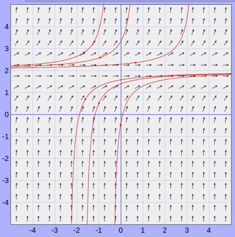
Example 66 .
Discuss the stability of the critical point(s) of the model.
\(\frac{dx}{dt}=(x-3)^2\text{.}\)
A slope field for
\(\frac{dx}{dt}=(x-3)^2\text{.}\)
The Effect of Parameters - Bifurcation. Parameters can have a significant effect on the type of solutions you obtain for a differential equation. For example, parameters can affect critical points.
Example 67 . Bifurcation point.
(Based on Number 21 from Section 2.2 of your textbook by Edwards, et.al.)
Consider the model
\begin{gather}
\frac{dx}{dt}=kx-x^3=-x(x^2-k)\tag{†}
\end{gather}
with parameter \(k\text{.}\)
If
\(k>0\text{,}\) then
(†) has
critical points:
.
If
\(k < 0\text{,}\) then
(†) has only
critical points:
.
We call
\(k=0\) a
point of the differential equation in
(†) because it is the point at which the parameter
\(k\) changes the
nature of the solutions.
We can visualize this by plotting all points
\begin{equation*}
(k,c)
\end{equation*}
such that
\(c\) is a critical point of
(†) for that value of
\(k\text{.}\)
A Cartesian coordinate system with independent variable \(k\) and dependent variable \(c\text{.}\)
Harvesting Logistic Populations.
Consider the logistic model that has been slightly modified to account for harvesting of a population (such as fishing or butchering beef).
\begin{align*}
\frac{dP}{dt} & = kP(M-P)-h \\
& = -kP^2+kMP-h
\end{align*}
where \(k, M, h>0\) and \(h\) represents the rate at which the population is being harvested.
\(kP(M-P)-h\) \(P\text{,}\)
The quadratic equation has 2 distinct real roots \(H\) and \(N\) with \(H<N\text{.}\) Using the quadratic formula, it can be argued that \(0 < H < N < M\text{.}\) (See example 4 in section 2.2 of your textbook by Edwards, et.al.)
There is one distinct real root \(N\text{.}\)
There are no real roots.
\begin{equation*}
\frac{dP}{dt}= -kP^2+kMP-h
\end{equation*}
Let’s consider the harvesting model
\begin{equation*}
\frac{dP}{dt}=P(6-P)-h = -P^2+6P-h
\end{equation*}
where \(k=1\) and \(M=6\text{.}\) Let’s look at what happens for some values of \(h\text{.}\) The direction fields on this page were made Ariel Barton’s direction field plotter. The graphs of parabolas were created using Desmos.
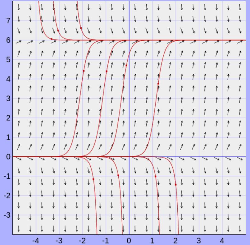
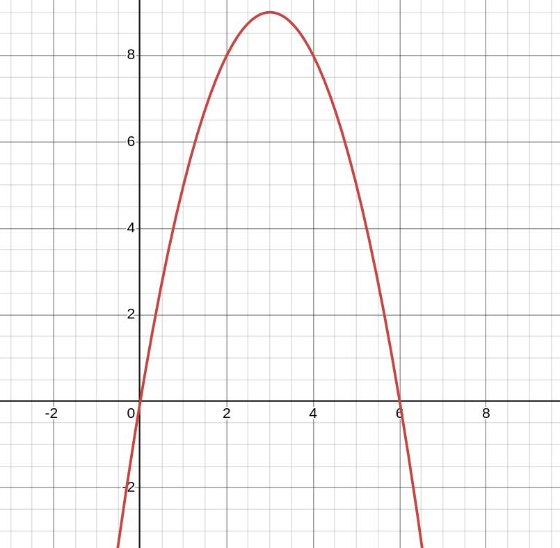
\(h=0\) (This is just a logistic growth model)
Slope field when harvesting rate is 0.
Graph of
\(y=-P^2+6P-0\text{.}\)
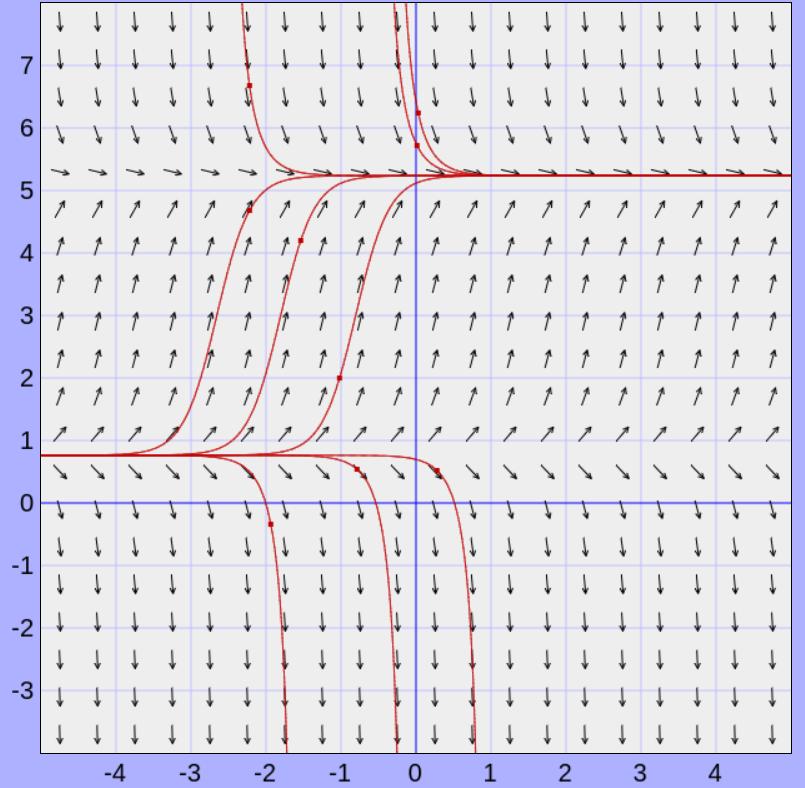
\(h=4\)
Slope field when harvesting rate is 4.
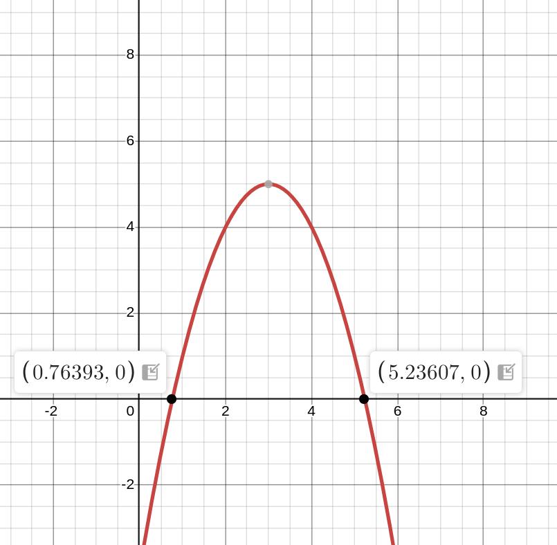
Graph of
\(y=-P^2+6P-4\text{.}\)
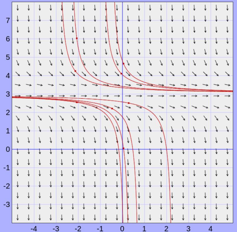
\(h=9\)
Slope field when harvesting rate is 9.
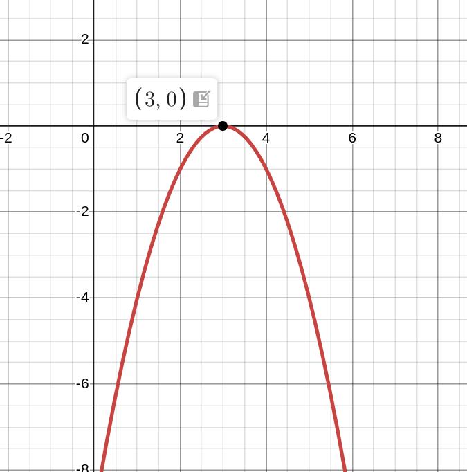
Graph of
\(y=-P^2+6P-9\text{.}\)
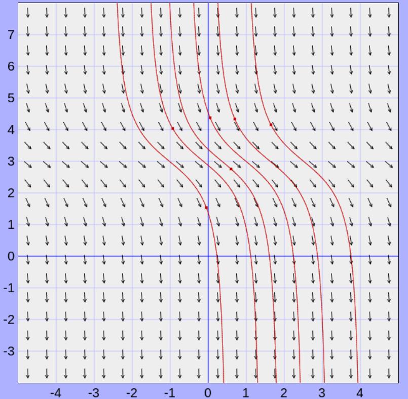
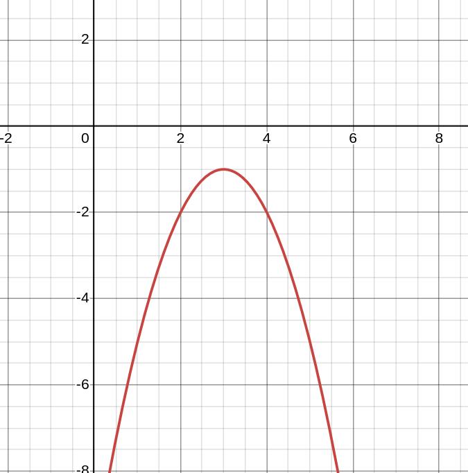
\(h=10\)
Slope field when harvesting rate is 10.
Graph of
\(y=-P^2+6P-10\text{.}\)