Find the position function, \(x(t)\text{,}\) for an undamped spring system if \(m=1\text{,}\) \(k=144\text{,}\) \(F(t)=88\cos(10t)\text{,}\) \(x(0)=0\text{,}\) and \(x'(0)=0\text{.}\)
Print preview
Handout Lessons 20 and 21, Forced Oscillations and Resonance
Textbook Section(s).
This lesson is based on Section 3.6 of your textbook by Edwards, Penney, and Calvis.
External Forces on Springs.
In Lesson 17, we developed a differential equation for a horizontal spring system in which a mass \(m\) was attached to a spring with spring constant \(k\) and a dashpot with damping constant \(c\text{.}\) We also considered the possibility that an external force \(F_E(t)\text{,}\) or simply \(F(t)\) was applied to the system. Our equation was:
\begin{gather}
mx''+cx'+kx=F(t)\tag{✶}
\end{gather}
The following diagram for a system of this type was taken from section 3.4 of your textbook. 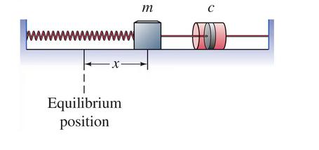
In Lesson 17, we only considered situations in which \(F_E(t)=0\text{.}\) In Lessons 20 and 21, we will consider what happens when an external force is applied to the spring, i.e., \(F(t) \neq 0\text{.}\) This application produces a nonhomogeneous linear differential equation with constant coefficients. Thus, the techniques from Lessons 18 and 19 provide tools for solving these application problems.
In Lessons 20 and 21, we will consider a specific type of external force, namely a simple harmonic external force. Some examples of a simple harmonic force include machines with spinning parts such as a washing machine or a dryer or the cadence of soldiers crossing a bridge. Simple harmonic forces can be modeled by:
\begin{gather}
F(t)=F_0\cos(\omega t)\tag{✶}
\end{gather}
or
\begin{gather}
F(t)=F_0\sin(\omega t)\tag{✶✶}
\end{gather}
Undamped Forced Oscillations, \(c=0\).
We start with the simplest case in which the spring in our system is undamped. In other words, \(c=0\) and our equation simplifies to:
\begin{gather}
mx''+kx=F_0\cos(\omega t)\tag{#}
\end{gather}
We start by finding the complementary solution, \(x_c=x_c(t)\) to (#) (i.e., the solution to the associated homogeneous equation).
If we set \(\omega_0=\sqrt{\frac{k}{m}}\text{,}\) then we have
Case 1: \(\omega_0 \neq \omega\).
In this case, the natural oscillation of the system differs from the oscillation introduced by the external force. Using the method of undetermined coefficients to solve
\begin{gather*}
mx''+kx=F_0\cos(\omega t)
\end{gather*}
our initial guess for the particular solution is
\begin{gather*}
x_p=A\cos(\omega t)+B\sin(\omega t)
\end{gather*}
Because there is no \(x'\) term in the equation and no sine function on the right-hand side, it is clear that \(B=\fillinmath{XXXXXXXXXX}\text{,}\) so we can simplify the guess for \(x_p\) to
\begin{gather*}
x_p=\fillinmath{XXXXXXXXXXXXXXXXXXXXXXXXXXXXXX}
\end{gather*}
Now we can solve for \(A\text{.}\)
We have an overall solution of
\begin{gather*}
x(t)=C\cos(\omega_0 t-\theta)+
\frac{F_0}{m(\omega_0^2-\omega^2)}\cos(\omega t)
\end{gather*}
Example 137. An undamped spring model where \(\omega \neq \omega_0\).
In the last example, our solution was
\begin{gather*}
x(t)=-2\cos(12t)+2\cos(10t)
\end{gather*}
which is the sum of two oscillations with periods:
The overall period of \(x(t)\) is .
Now let’s use the sum-to-product identity
\begin{gather}
\cos(\alpha)-\cos(\beta)=-2\sin\left(\frac{\alpha-\beta}{2}
\right)\sin\left(\frac{\alpha+\beta}{2} \right)\tag{#}
\end{gather}
to examine our solution.
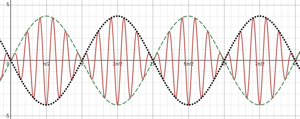
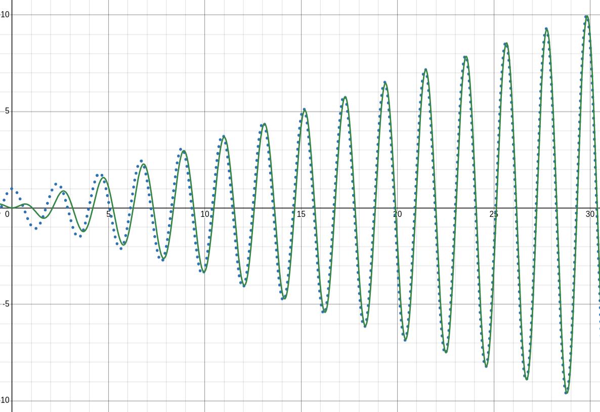
The red solid graph is
\begin{gather*}
x(t)=-2\cos(12t)+2\cos(10t)=4\sin(t)\sin(11t)
\end{gather*}
The green dashed graph is
\begin{gather*}
x(t)=4\sin(t)
\end{gather*}
The black dotted graph is
\begin{gather*}
x(t)=-4\sin(t)
\end{gather*}
Case 2: \(\omega_0 = \omega\).
Remember that we are still dealing with undamped systems in which a simple harmonic force is applied. In this case, the natural oscillation of the system is identical to the oscillation introduced by the external force. This produces resonance.
Example 138. An undamped spring model as \(\omega \rightarrow \omega_0\).
Recall that when \(\omega \neq \omega_0\text{,}\) then the position function of our spring is given by
\begin{gather*}
x(t)=C\cos(\omega_0 t-\theta)+
\frac{F_0}{m(\omega_0^2-\omega^2)}\cos(\omega t)
\end{gather*}
Let’s use Desmos to see what happens as \(\omega \rightarrow
\omega_0\text{.}\) In all of the graphs below \(\omega_0=3\text{.}\) I will vary the value of \(\omega\text{.}\)

You can use the Desmos graph to see what happens with other values of \(\omega\text{.}\) I encourage you to try values of \(\omega\) that are approaching \(3\) from the left. The pictures on this pageonly approach \(3\) from the right.
Finding solutions when we have resonance.
Now, let’s find the solution for our spring equation when \(\omega=\omega_0\)
\begin{gather}
mx''+kx=F_0\cos(\omega_0 t)\tag{†}
\end{gather}
We still have the complementary solution
\begin{gather*}
x_c=c_1\cos(\omega_0 t) +c_2\sin(\omega_0 t)
\end{gather*}
but to prevent duplication with the complementary solution, we adjust the form of our particular solution to be
\begin{gather*}
x_p=\fillinmath{XXXXXXXXXXXXXXXXXXXXXXXXXXXXXX}
\end{gather*}
Then using the method of undetermined coefficients, we can find the particular solution
\begin{gather*}
x_p=\frac{F_0}{2m\omega_0}t\sin(\omega_0 t)
\end{gather*}
If we set
\begin{gather*}
A(t)=\frac{F_0}{2m\omega_0}t
\end{gather*}
then \(|A(t)| \rightarrow \fillinmath{XXXXXXXXXX}\) as \(t \rightarrow \infty\text{.}\)
Example 139.
For an undamped spring system with \(\omega=\omega_0\text{,}\) we have the solution
\begin{align*}
x(t) \amp = c_1\cos(\omega_0 t) +
c_2\sin(\omega_0 t) + \frac{F_0}{2m\omega_0}t
\sin(\omega_0 t )\\
\amp = C\cos(\omega_0 t - \alpha) +
\frac{F_0}{2m\omega_0}t\sin(\omega_0 t )
\end{align*}
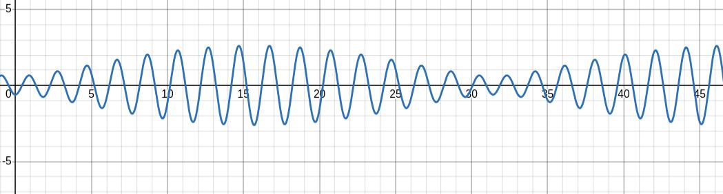
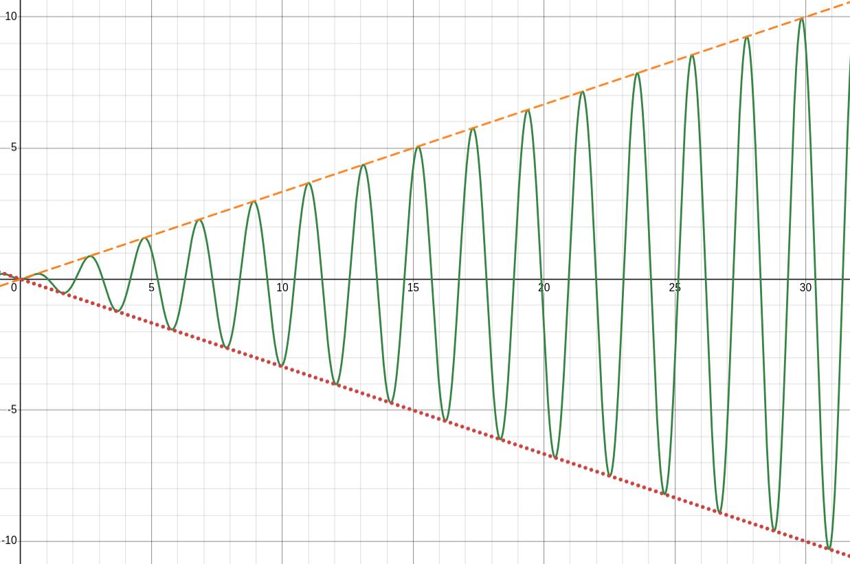
In the Desmos graphs below, \(\omega=\omega_0=3\text{,}\) \(C=1\text{,}\) \(\alpha=0\text{,}\) \(m=1\text{,}\) and \(F_0=2\text{.}\)
In the first graph, the dashed blue graph is the overall solution.
\begin{equation*}
x(t) = C\cos(\omega_0 t - \alpha) +
\frac{F_0}{2m\omega_0}t\sin(\omega_0 t).
\end{equation*}
In both graphs, the green solid graph is just the particular solution.
\begin{equation*}
x_p(t) = \frac{F_0}{2m\omega_0}t\sin(\omega_0 t).
\end{equation*}
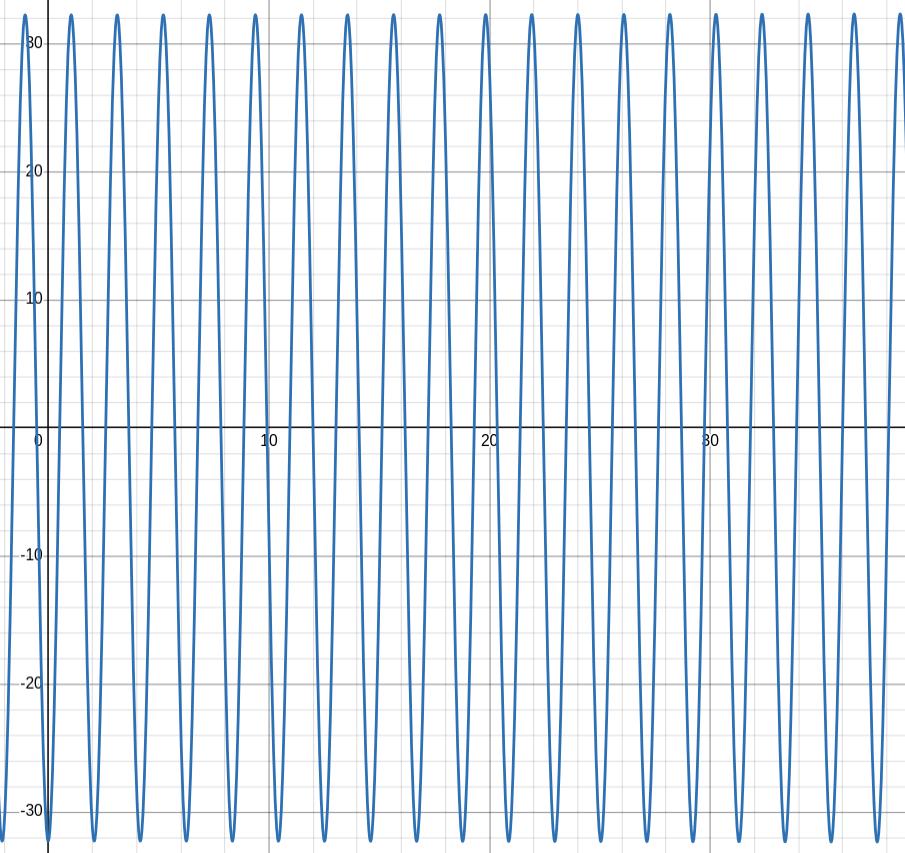
You can see from the first graph that the complementary solution has very little effect on the overall solution. The particular solution is dominating the behavior of the overall solution. In the second graph, the orange dashed graph is the amplitude function
\begin{equation*}
A(t) = \frac{F_0}{2m\omega_0}t
\end{equation*}
and the red dotted graph is the negative of the amplitude function
\begin{equation*}
-A(t) = -\frac{F_0}{2m\omega_0}t\text{.}
\end{equation*}
You can see the amplitude exploding in the second graph.
Damped, Forced Oscillations, \(c\neq 0\).
We are now working with spring equation of the form
\begin{gather}
mx''+cx'+kx=F_0\cos(\omega t)\tag{##}
\end{gather}
The characteristic equation associated with (##) is which has solutions
\begin{gather*}
r=-\frac{c}{2m} \pm \frac{\sqrt{c^2-4km}}{2m}.
\end{gather*}
Notice that if \(c^2-4km > 0\text{,}\) then \(\sqrt{c^2-4km} \lt c\text{,}\) so that if the characteristic equation has 2 real roots, then both roots are .
Complementary solutions for damped, forced oscillations.
The characteristic equation for (##) has two complex solutions, one real solution of multiplicity 2, or two distinct real solutions. This leads to three possibilities for the complementary solutions.
| Damping type | \(x_c=x_{tr}\text{,}\) transient solutions |
|---|---|
| underdamped | \(x_c=e^{-\frac{ct}{2m}}\left(\widehat{A}\cos(\mu t)+ \widehat{B}\sin(\mu t) \right) = Ae^{-\frac{ct}{2m}} \cos(\mu t - \theta)\) |
| critically damped | \(x_c=c_1e^{rt}+c_2te^{rt}, r=-\frac{c}{2m}\) |
| overdamped | \(x_c = c_1e^{r_1t}+c_2e^{r_2t}\) (\(r_1\) and \(r_2\) distinct negative real roots) |
Because of the negative exponents, in all three cases, \(x_c(t) \rightarrow \fillinmath{XXXXXXXXXX}\) as \(t \rightarrow \infty\text{.}\)
Particular solutions for damped, forced, oscillations.
Because the complementary solutions in the damped case have virtually no impact as time passes, the particular solutions dominate the behavior of the spring system. In the damped case, the particular solutions are called the steady periodic solutions and are sometimes denoted \(x_{sp}\text{.}\) Using the method of undetermined coefficients, our first guess for the form of the particular solution for
\begin{gather}
mx''+cx'+kx=F_0\cos(\omega t)\tag{#}
\end{gather}
would be
\begin{gather*}
x_{sp}=A\cos(\omega t)+B\sin(\omega t).
\end{gather*}
Fortunately, there is no overlap with \(x_c=x_{tr}\text{,}\) so we proceed as normal.
-
Take derivatives of \(x_{sp}\) and plug into (#).
-
Equate coefficients and solve for \(A\) and \(B\text{.}\)
-
Convert our solutions for \(x_{sp}\) into a form only involving cosine.
You are encouraged to find that
\begin{gather*}
x_{sp}=\frac{F_0}{\sqrt{(k-m\omega^2)^2+c^2\omega^2}}
\cos(\omega t - \theta).
\end{gather*}
Combining this with the complementary, transient solution gives the general solution
\begin{align}
\tag{#}
\end{align}
Amplitude and practical resonance for damped, forced, oscillations.
The forced amplitude function, \(C(\omega)\) is defined to be
\begin{gather*}
C(\omega)= \frac{F_0}{\sqrt{(k-m\omega^2)^2+
c^2\omega^2}}
\end{gather*}
Notice that the denominator of \(C(\omega)\) never equals so there is no pure when we have damping.
Definition 141.
In a damped spring system, practical resonance occurs at the positive \(\omega\) value that maximizes
\begin{gather*}
C(\omega)= \frac{F_0}{\sqrt{(k-m\omega^2)^2+
c^2\omega^2}}
\end{gather*}
provided that \(C(\omega)\) has a maximum value on \((0, \infty)\text{.}\) If \(C(\omega)\) has a maximum value on \((0, \infty)\text{,}\) then we denote the \(\omega\) value where the maximum occurs by \(\omega_{\text{max}}\) and call \(\omega_{\text{max}}\) the practical resonance frequency.
Example 142. Practical resonance.
In Example 6 from Section 3.6 of your textbook, they consider a spring system with \(m=1\text{,}\) \(c=2\text{,}\) \(k=26\text{,}\) and \(F_0=82\text{,}\) resulting in the equation
\begin{gather*}
x''+2x'+26x=82\cos(\omega t).
\end{gather*}
Using the method of undetermined coefficients, we look for a particular solution of the form
\begin{gather*}
x_p=x_{sp}=A\cos(\omega t)+B\sin(\omega t)
\end{gather*}
and are able to find the
\begin{align*}
x_{sp} \amp = \frac{(26-\omega^2)(82)}
{(26-\omega^2)^2+(2\omega)^2}\cos(\omega t) +
\frac{2\omega(82)}{(26-\omega^2)^2+(2\omega)^2}
\sin(\omega t)\\
\amp = C(\omega)\cos(\omega t - \alpha)
\end{align*}
We want to understand the practical resonance, so we look at
\begin{align*}
C(\omega) \amp = \sqrt{A^2+B^2}\\
\amp = \frac{82}{\sqrt{(26-\omega^2)^2+
(2\omega)^2}}
\end{align*}
The maximum of \(C(\omega)\) occurs when . . .
Amplitude of practical resonance frequency:
This graph may help you to understand the results of the previous example.
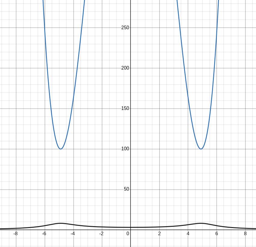
The graph of \(g(\omega)=(26-\omega^2)^2+(2\omega)^2\) and the graph of \(C(\omega)=\frac{82}{\sqrt{(26-\omega^2)^2+(2\omega)^2}}\text{.}\) The minimum of \(g\) occurs at the same \(\omega\) value where the maximum of \(C\) occurs.
