Let’s take a step back in time to your Calculus I class. One of the concepts that you are supposed to glean from your Calculus I class is that if the function \(f\) is differentiable at \(x_0\) and \(L(x)\) is the equation for the tangent line to \(f\) at \(x_0\text{,}\) then
\begin{equation*}
f(x_1) \approx L(x_1)
\end{equation*}
if \(x_1\) is sufficiently close to \(x_0\text{.}\) This is the idea behind linear approximations. (This is also the first step in using Taylor polynomials to approximate function values.)
Example 70.
Use a linear approximation to estimate
\(\sqrt{4.1}\text{.}\)

The graph of \(y=f(x)=\sqrt{x}\) and its tangent line at \((4,2)\text{.}\)
Euler’s Method is used to approximate points on the solution curve of an IVP.
\begin{gather}
\frac{dy}{dx}=f(x,y), \qquad y(x_0)=y_0\tag{✶}
\end{gather}
We are interested in the function
\begin{equation*}
y(x)
\end{equation*}
which is a solution of
(✶). Unlike linear approximation problems, we do not have the function (unless it is a really special differential equation that is easy to solve). We only have its derivative. Because the IVP provides us with the point
\((x_0,y_0)\text{,}\) the derivative is all we need to find an equation for the tangent line to the solution curve through this point. We will then use that tangent line to approximate the
\(y\)-value of the point on the solution curve at
\(x=x_1=x_0+h\text{,}\) for some small
\(h\) value. This new point,
\((x_1,y_1)\) probably is not on the solution curve,
\(y=y(x)\text{,}\) but we hope that it is close to the solution curve. So we pretend that it is on the solution curve, use the derivative we are given in the IVP to construct a "tangent line" to
\(y=y(x)\) "at"
\((x_1,y_1)\text{,}\) and use this "tangent line" to approximate the
\(y\)-value of the point on the solution curve at
\(x=x_2=x+2h\text{.}\) The process continues until you reach a desired stopping point.
The picture below is Figure 2.4.1 of your textbook by Edwards, et.al.
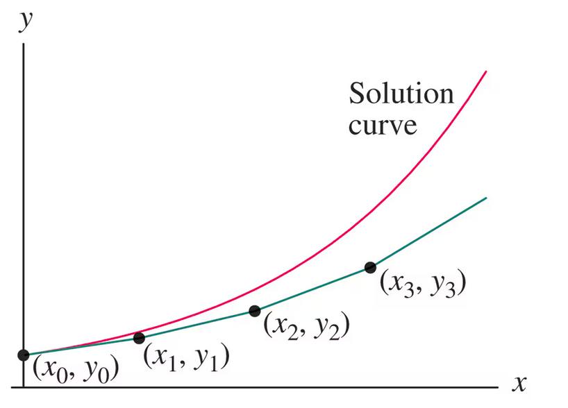
A picture of the solution curve for an IVP and the Euler approximation curve. The Euler approximation curve is a piecewise linear curve connecting the Euler approximation points. In this example, only
\((x_0, y_0)\) is on the solution curve. There are errors in the other approximation points.
Example 72. Using Euler’s method.
(Based on Number 7 from Section 2.4 of your textbook by Edwards, et.al.)
Use Euler’s method with step size 0.2 to find \(y_1\) and \(y_2\) for the IVP.
\begin{equation*}
\frac{dy}{dx}=-3x^2y, \qquad y(0)=3
\end{equation*}
Let’s use MATLAB to verify our results. The department has provided a MATLAB file
eul.m that you may use. It is on the course website. I have also posted it in the Extra Resources module for our course in Brightspace.
To begin, I created a text file for my function named
fcn1.m. The contents of that file are shown below.
function W=fcn1(x,y)
W=-3*x^2*y;
In a terminal, I navigated to the directory that contained
eul.m and
fcn1.m. I then ran the following commands:
>> [x,y]=eul('fcn1',[0,0.4],3,0.2);
>> [x,y]
ans =

         0    3.0000
    0.2000    3.0000
    0.4000    2.9280
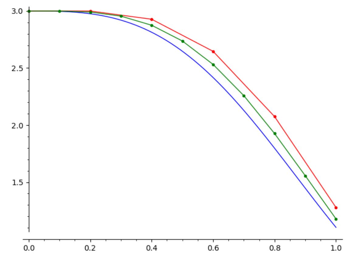
For the IVP
\begin{equation*}
\frac{dy}{dx}=-3x^2y, \qquad y(0)=3\text{,}
\end{equation*}
I have graphed the solution curve \(y(x)=e^{-x^3}\text{,}\) the Euler approximation curve on \([0,1]\) using \(h=0.2\text{,}\) and the Euler approximation curve using \(h=0.1\text{.}\)
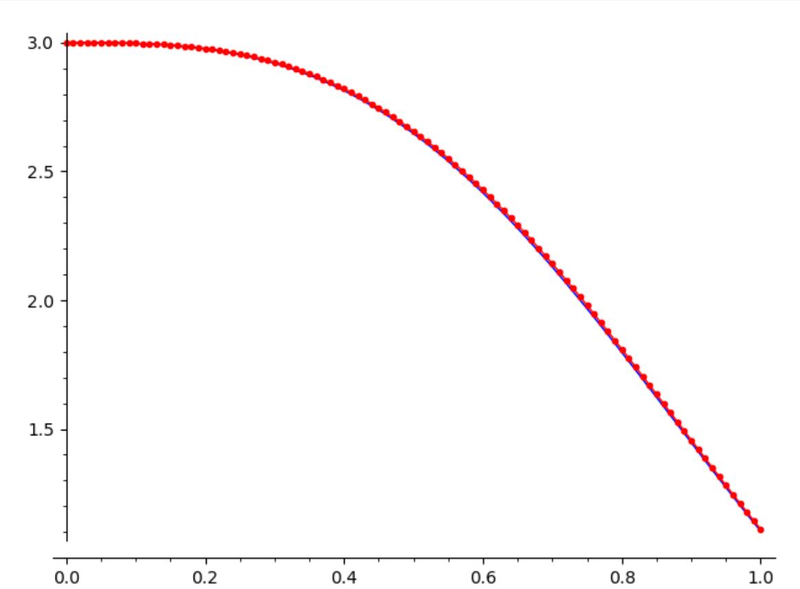
In the next picture, I have graphed the solution curve
\(y(x)=e^{-x^3}\) and the Euler approximation curve on
\([0,1]\) using
\(h=0.01\text{.}\)
The picture below is Figure 2.5.3 in your textbook by Edwards, et.al. It is used to explain the Improved Euler Method Algorithm for approximating points on the solution curve of an IVP.
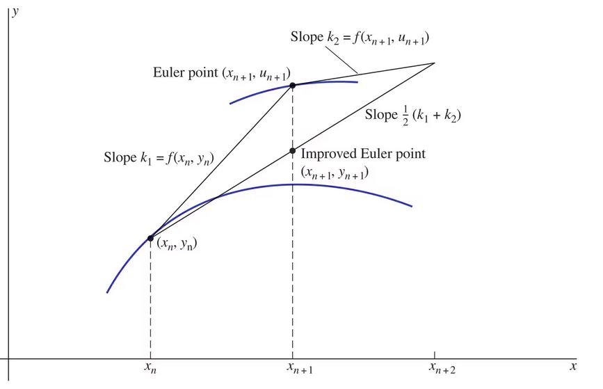
The starting point, the Euler point, and the improved Euler point
Algorithm 73. Improved Euler Method for Approximating Solutions for IVP’s.
Given:
-
An IVP
\begin{equation*}
\frac{dy}{dx}=f(x,y), \qquad y(x_0)=y_0
\end{equation*}
-
A step size \(h \neq 0\)
Return: A list \([y_0, y_1, y_2, y_3, \dots, ]\) using the following algorithm:
-
\(x_n = x_0+nh\text{,}\) \(x_{n+1}=x_0+(n+1)h\)
-
\(\displaystyle k_1=f(x_n,y_n)\)
-
\(\displaystyle u_{n+1}=y_n+hk_1\)
-
\(\displaystyle k_2=f(x_{n+1},u_{n+1})\)
-
\(\displaystyle y_{n+1} = y_n+h\frac{1}{2}(k_1+k_2)\)
for \(n \in \set{1, 2, 3, \dots}\text{.}\)
For the IVP
\begin{equation*}
\frac{dy}{dx}=x-y, \qquad y(0)=1\text{,}
\end{equation*}
I have graphed the solution curve \(y(x)=2e^{-x}+x-1\text{,}\) the Euler approximation curve, and the improved Euler approximation curve both on \([0,1]\) and using \(h=0.1\text{.}\)
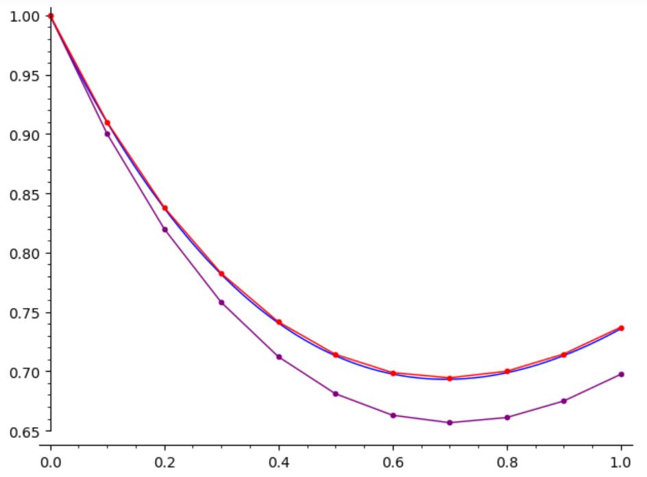
The error is evident between the solution curve and the Euler approximation. The error between the solution curve and the improved Euler approximation is almost indistinguishable.
Approximations are not perfect. Here are a couple of potential pitfalls for the Euler Method and the Improved Euler Method.