This lesson is based on Section 1.3 of your textbook by Edwards, Penney, and Calvis.
Geometric Approach to Approximating Solutions of Differential Equations.
In the Lesson 1, I gave you a function and asked you to verify that it was a solution to a differential equation. In Lesson 2, I asked you to use Calculus to solve some differential equations of the form
\begin{equation*}
\frac{dy}{dx}=f(x)
\end{equation*}
Today we will look at differential equations of the form
\begin{equation*}
\frac{dy}{dx}=f(x,y).
\end{equation*}
This problem can be much more complicated than what you might imagine. The authors of your textook (Edwards, Penney, and Calvis) tell you that even the seemingly benign differential equation
\begin{equation*}
\frac{dy}{dx}=x^2+y^2
\end{equation*}
cannot be solved using elementary functions.
In my mind, one of the major themes of calculus is the following:
If you do not know how to find an exact solution, do what you can to find an approximation.
While it can be argued that graphical methods do not provide proofs of mathematical results, they do provide intuition and approximations. Intuition is key to much mathematical insight. Today we are going to explore
slope fields, a graphical approach that will hopefully give us some insight into the solutions of a differential equation.
Recall that
\(\frac{dy}{dx}\) is a formula for finding the
\(\spc{2in}\) of the tangent line to a curve at a given point. A
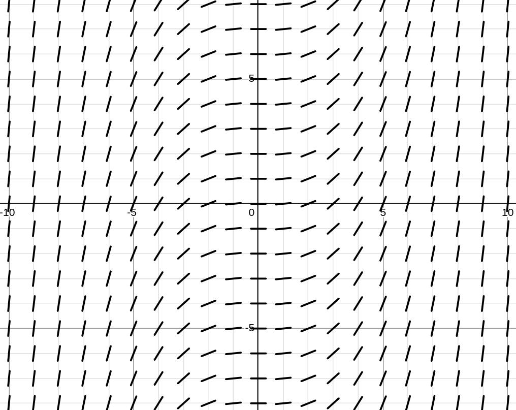
slope field is a graph that contains tiny tangent segments for curves that satisfy the differential equation. When you plot enough of these tangent segments, you can very often get a good feel for what the solution curves look like.
Let’s start with a simple example that we could solve using the techniques in Lesson 2. It will help us to better understand this new technique.
NOTE I used Darryl Nester’s website to construct all of the remaining slope fields in these notes. Sometimes slope fields can help us to understand trends for solution curves. Consider two different population models.
Definition 18. The Exponential Growth Model.
A population grows exponentially if its rate of increase is proportional to the size of the population.
\begin{equation*}
\frac{dP}{dt} = kP
\end{equation*}
where \(k\) is a constant.
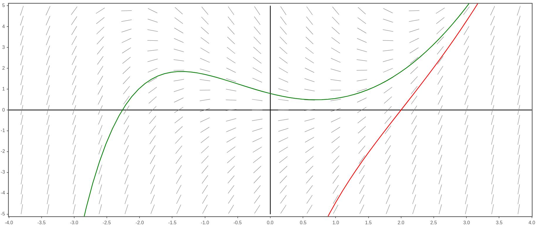
Here is a slope field for the exponential growth model
\begin{equation*}
\frac{dP}{dt}=P\text{.}
\end{equation*}
(Notice that
\(k=1\text{.}\))
Slope field and some solution curves showing exponential growth
Can you see why this is called an exponential growth model?
Definition 19. The Logistic Growth Model.
A population grows logistically with carrying capacity \(M\) if it satisfies the differential equation
\begin{equation*}
\frac{dP}{dt} = kP\left(1-\frac{P}{M}\right)
\end{equation*}
where \(k\) is a constant.
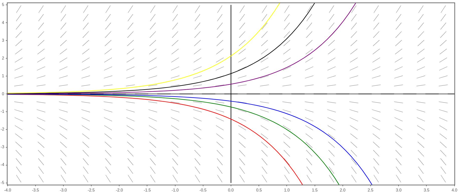
Here is a slope field for the logistic growth model
\begin{equation*}
\frac{dP}{dt}=P\left(1 -\frac{P}{6}\right)\text{.}
\end{equation*}
(In this model,
\(P\) is measred in thousands. Once again, note that
\(k=1\text{.}\))
Slope field and some solution curves of showing logistic growth
What does this slope field tell you about this particular growth model?
Earlier in this course, we considered a fairly simple model for the acceleration of a falling object based only on the acceleration due to gravity. Now, let’s tweak that model to assume that gravity is pulling the object down, but the air resistance is pushing the object up. If we assume that the positive \(y\)-axis is pointing downward, this leads to a differential equation model of the form
\begin{equation*}
\frac{dv}{dt}=g-kv
\end{equation*}
where \(g\) is the acceleration constant due to gravity and \(k\) is a proportinality constant due to the wind resistance.
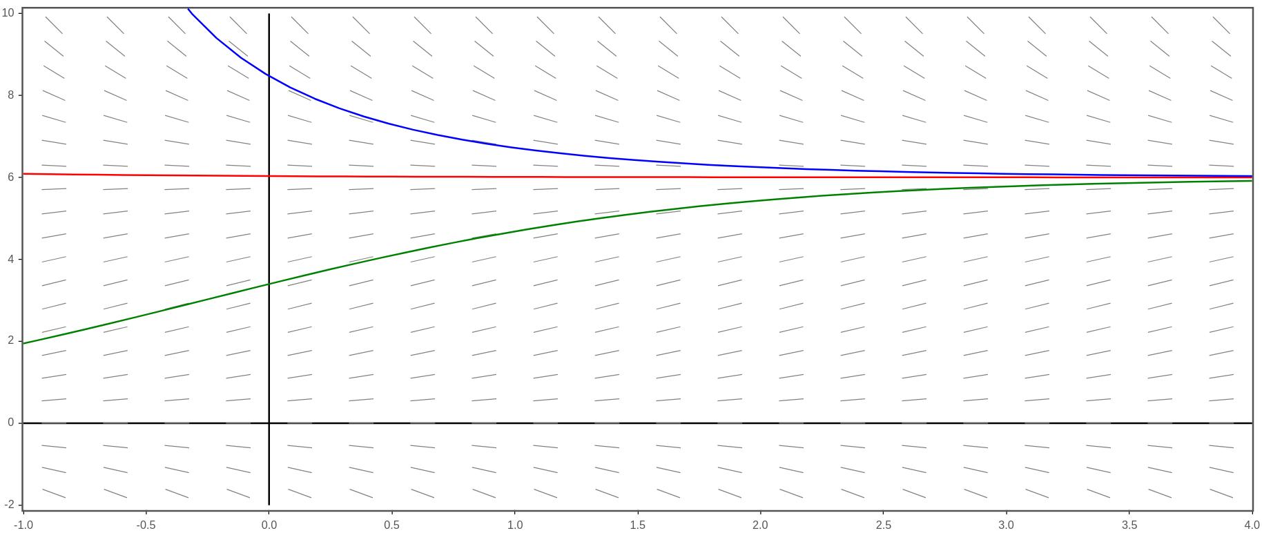
Suppose that \(k=0.5\) and we are using English units (ft, sec, etc). The differential equation would be
\begin{equation*}
\frac{dv}{dt}=32-0.5v
\end{equation*}
The slope field is shown below.
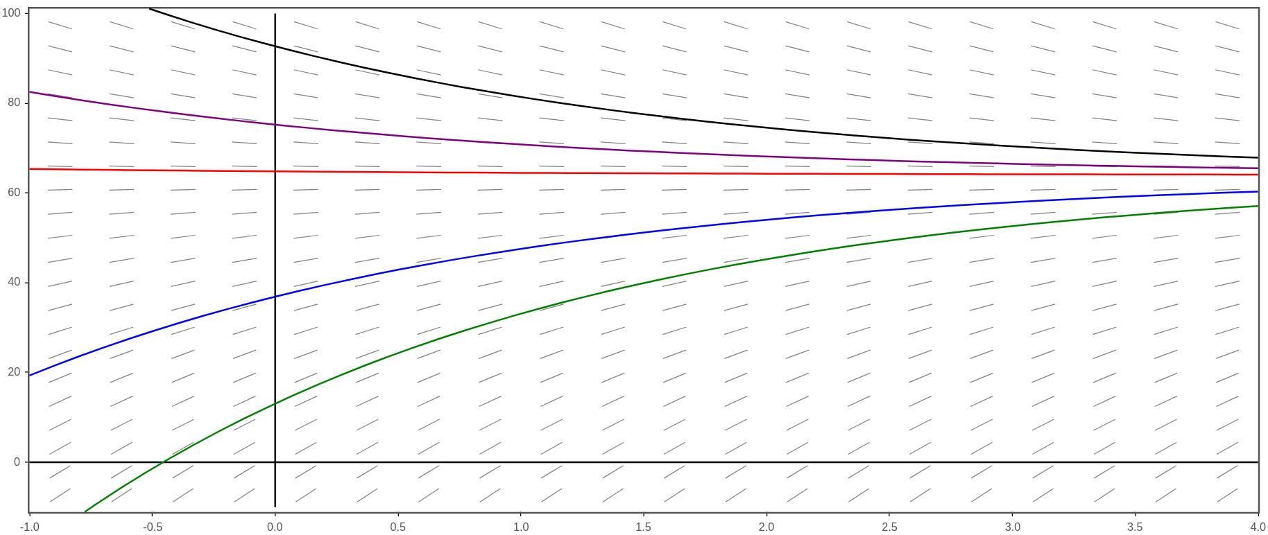
Slope field modeling a falling object and some solution curves
Can you see that no matter the initial velocity, if given enough time, the velocity will approach $64$ ft/s?
Existence and Uniqueness of Solutions of IVPs.
Not every IVP has a solution. Furthermore, those IVP’s that have solutions do not always have unique solutions.
Theorem 20. Existence and Uniqueness.
If both \(f(x,y)\) and \(D_y f(x,y)\) are continuous on some rectangle \(R\) that contains the point \((a,b)\) in the interior, then there is an interval \(I\) containing \(a\) for which the inital value problem
\begin{equation*}
\frac{dy}{dx}=f(x,y), \qquad y(a)=b
\end{equation*}
has a unique solution on the interval \(I\text{.}\)
Example 21. When existence and uniqueness fails.
-
Explain why the initial value problem does not have a solution.
\begin{equation*}
y\frac{dy}{dx}-4x=0, \qquad y(3)=0
\end{equation*}
-
Show that
\begin{equation*}
y_1= 2x
\end{equation*}
and
\begin{equation*}
y_2= -2x
\end{equation*}
are both solutions of the initial value problem
\begin{equation*}
y\frac{dy}{dx}-4x=0, \qquad y(0)=0
\end{equation*}