Systems of Differential Equations.
Definition 143.
A
system of differential equations is a set of differential equations.
A
solution of a system of differential equations is a set of functions that satisfy
all of the differential equations in the system over some interval of the independent variable.
Example 144. Verifying a solution of a system of differential equations.
(Based on Number 23 from Section 4.1 of your textbook by Edwards, et.al.)
Consider the system of differential equations
\begin{align}
\begin{cases}
x' \amp = y \\
y' \amp = 6x-y
\end{cases}\tag{#}
\end{align}
The independent variable for this system is
. Verify that
\(x(t)=e^{2t}\text{,}\) \(y(t)=2e^{2t}\) is a solution of the system of differential equations in
(#).
Systems of differential equations arise from:
-
-
mixing problems with multiple tanks
-
spring problems with multiple springs
Converting a differential equations into a system of first-order differential equations.
There are computer algorithms for solving systems of first-order differential equations. Therefore, if we can convert a single differential equaiton in to a system of first-order differential equations, then we can use the computer to solve higher order differential equations.
Example 147. Converting a higher order DE into a system of first order DE’s.
Find a system of first-order differential equatons that is equivalent to
\begin{gather}
x^{(4)}+2x^{(3)}-x=e^{5t}\tag{†}
\end{gather}
General Procedure: Convert
\begin{gather}
x^{(n)}=f(t,x,x', \dots, x^{(n-1)})\tag{✶}
\end{gather}
to
\begin{align}
\begin{cases} x_1' \amp = x_2 \\ x_2' \amp = x_3 \\ \amp \vdots \\
x_{n-1}' \amp = x_n \\ x_n' \amp = f(t,x_1,x_2, \dots, x_n)
\end{cases}\tag{✶✶}
\end{align}
Solve
(✶✶). Then
\(x(t)=x_1(t)\) is a solution of
(✶).
Example 148. Converting a system of higher order DE’s into a systemm of first order DE’s.
(Number 10 from Section 4.1 of your textbook by Edwards, et.al.)
Transform the system of differential equations into an equivalent system of first-order differential equations.
\begin{align*}
\begin{cases} x''-5x+4y \amp = 0 \\ y''+4x-5y \amp = 0
\end{cases}
\end{align*}
Solving two-dimensional systems of differential equations.
We now turn our attention to solving some systems of differential equations. In this course, we will focus on solutions of
two-dimensional systems of differential equations. These systems have two unknown functions. Normally we will denote these unknown fuctions by
\(x(t)\) and
\(y(t)\text{,}\) or just
\(x\) and
\(y\) for short. In this section of the notes, we will use a substitution approach and direction fields to help us understand the solutions of these systems of equations. In the last section of these notes, we will use the method of elimination to solve a special category of these systems of equations.
In the next example, we will use a substitution approach to solve a two-dimensional system of differential equations. As we are working through this problem, notice that the technique does not produce a clear-cut algorithm for solving these systems. It requires a bit of creativity and is very dependent on the equations in the system.
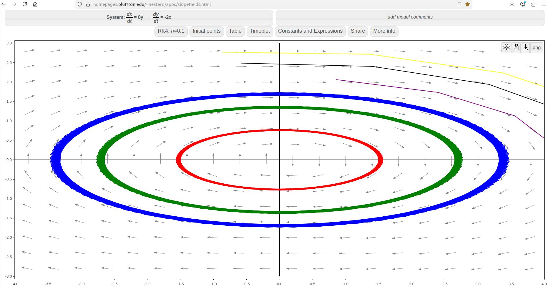
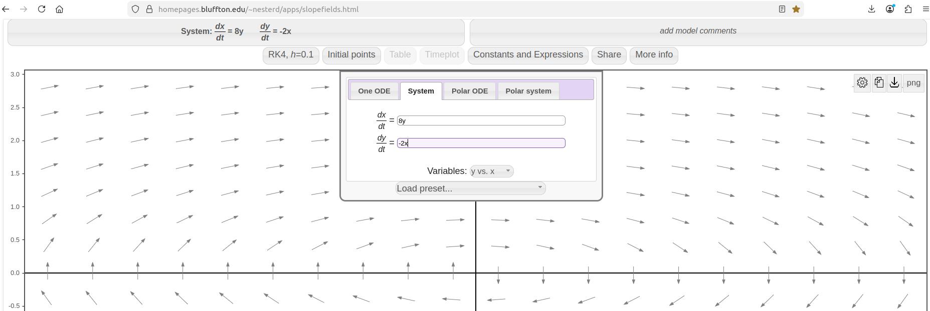
Example 149. Solving a system using substitution.
(Number 22 from Section 4.1 of your textbook by Edwards, et.al.)
Solve the system of differential equations.
\begin{align}
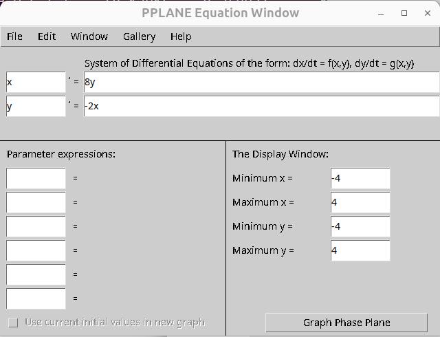
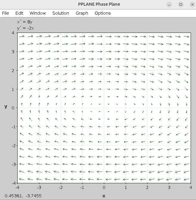
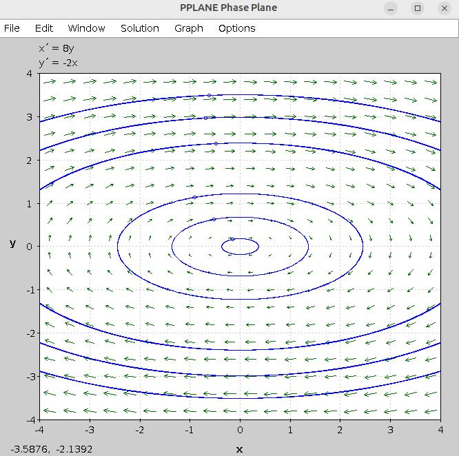
\begin{cases} x' \amp = 8y \\ y' \amp = -2x \end{cases}\tag{‡}
\end{align}
Using direction fields to understand solutions of two-dimensional systems of differential equations.
There are various programs for plotting direction fields of two-dimensional systems of differential equations. I will describe two of them in these notes.
Darryl Nester’s Slope and Direction Field Plotter.
-
-
Click on the
ODE. It will bring up a menu. Select the tab that says
System.
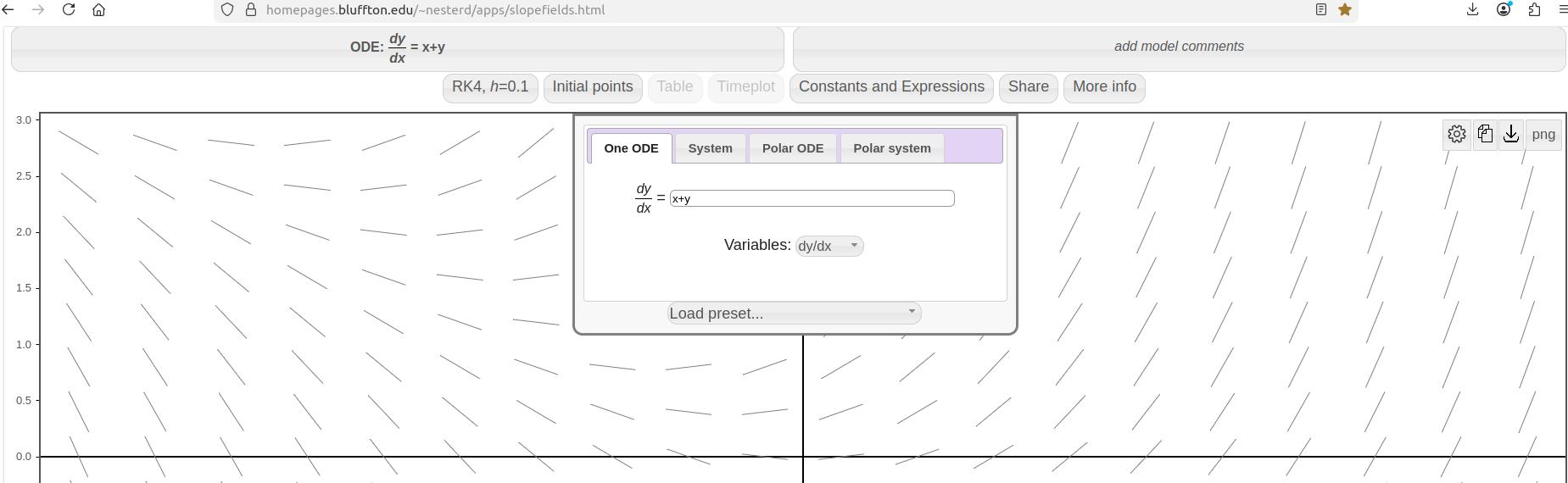
-
Enter the system of equations.
Solving systems of linear differential equations with constant coefficients by elimination.
In general, solving systems of differential equations can be difficult and may require some creativity. When the system contains only linear differential equations with constant coefficients, then we can apply the
Elimination Algorithm to solve the system. This is similar to the elimination method you used in high school to solve systems of linear equations.
-
Combine equations to eliminate unknown functions until you have a single differential equation containing only one unknown function.
-
Solve that equation for the unknown function.
-
Use that solution to help you find the other unknown functions.
This approach is more
than substitution or the direction field tools that we used previously. For those of you who have already done your supplemental work on section 5.1, you may notice that we are gearing up for some matrix notation soon. The
key to the elimination method is the behavior of
.
Proposition 151.
Let
\begin{equation*}
L_1 = a_nD^n+a_{n-1}D^{n-1}+ \dots + a_1D+ a_0
\end{equation*}
and
\begin{equation*}
L_2 = b_nD^n+b_{n-1}D^{n-1}+ \dots + b_1D+ b_0
\end{equation*}
be polynomial differential operators, then
\begin{gather*}
L_1L_2[x]=L_2L_1[x]
\end{gather*}
In general, differential operators do
commute. The fact that polynomial differential operators do commute is a very special case.
In this set of notes,
\(L_i\) will always refer to a polynomial differential operator.
The Elimination Algorithm can be used to solve a system of differential equations of the form
\begin{align}
\begin{cases}
L_1x+L_2y \amp = f_1(t) \\
L_3x+L_4y \amp = f_2(t)
\end{cases}\tag{✠}
\end{align}
We could spend a lot of time describing the algorithm, but I think that the algorithm becomes clear after you see a few examples.
Example 153. Solving systems of DE’s by elimination.
(Number 12 from Section 4.2 of your textbook by Edwards, et.al.)
Solve the system of differential equations.
\begin{align*}
\begin{cases} x'' \amp = 6x-2y \\ y'' \amp = -3x+7y
\end{cases}
\end{align*}
I would encourage you to take another look at number 22 from Section 4.1 of your textbook by Edwards, et. al. We did this problem in
Example 149. Can you use elimination to find the solution we found before?