When \(A\) is a \(2\times 2\) matrix, there are only three different types of solutions that \(\mathbf{x}'=A\mathbf{x}\) can have based on its eigenvalues and eigenvectors.
\(A\) has two distinct real eigenvalues (\(\lambda_1\) and \(\lambda_2\) with eigenvectors \(\mathbf{v_1}\) and \(\mathbf{v_2}\text{,}\) respectively.)
\(A\) has only one real eigenvalue (\(\lambda_1=\lambda_2\)) that yields two linearly independent eigenvectors \(\mathbf{v_1}\) and \(\mathbf{v_2}\text{.}\)
The solution curves in \(x_1x_2\)-space are dependent on the eigenvalues and eigenvectors. We will look at a few of these cases in depth. If we are not able to look at all of the cases, then I will refer you to your textbook.
Please note that unless otherwise stated, all of the pictures in this set of notes were created using Sagemath. Section 5.3 of your textbook by Edwards, Penney, and Calvis also has many helpful pictures.
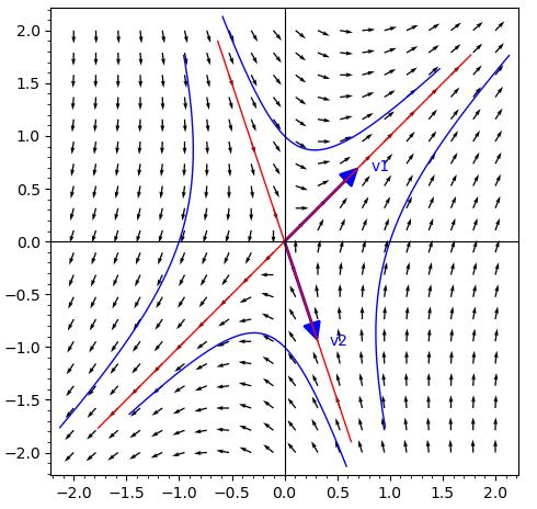
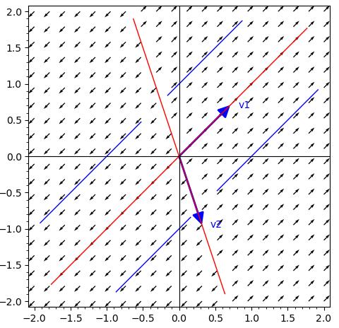
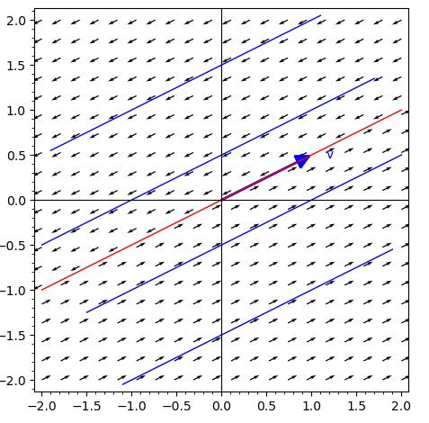
Case 1:\(A\) has two distinct real eigenvalues of opposite signs (\(\lambda_1
> 0\) and \(\lambda_2 < 0\) with eigenvectors \(\mathbf{v_1}\) and \(\mathbf{v_2}\text{,}\) respectively.)
This case produces a saddle point. In the picture below, \(\lambda_1>0\) and \(\lambda_2<0\text{.}\) The picture displays a vector field for a system with a positive eigenvalue and a negative eigenvalue. The eigenvectors are included and several solution curves. The solution curves move away from the line associated with the eigenvector for the negative eigenvalue and toward the line associated with the eigenvector for the positive eigenvalue.
A trajectory can be seen as a set of parametric equations describing a curve. Curves defined by parametric equations have directions, so we can place arrows on trajectories indicating how they are traversed as \(t\) increases.
I also want to note that your textbook says that a node is proper if “no two different pairs of ’opposite’ trajectories are tangent to the same straight line through the origin” and it is improper otherwise. Consequently, if at least four trajectories have the same tangent line at a node, then the node must be improper.
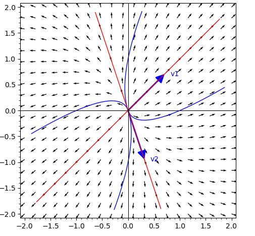
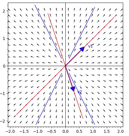
Case 2:\(A\) has two distinct positive eigenvalues (\(\lambda_1\) and \(\lambda_2\) with eigenvectors \(\mathbf{v_1}\) and \(\mathbf{v_2}\text{,}\) respectively.)
This case produces an improper nodal source. In the picture below, \(0<\lambda_2<\lambda_1\text{.}\) The picture displays a vector field for a system with two distinct positive eigenvalues The eigenvectors are included and several solution curves. The solution curves move away from the line associated with the eigenvector for the smaller eigenvalue and become more parallel to the line associated with the eigenvector for the larger eigenvalue.
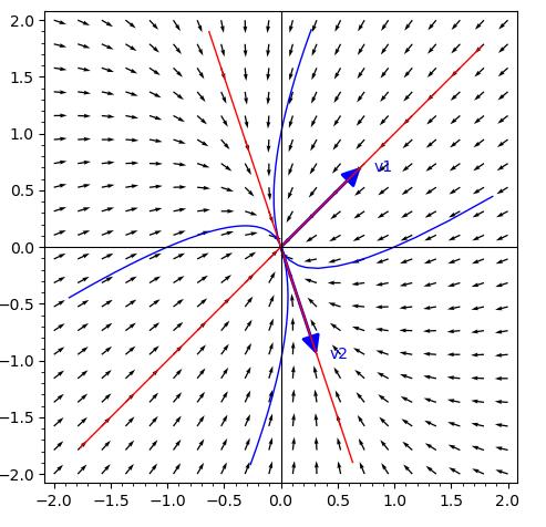
Case 3:\(A\) has two distinct negative eigenvalues (\(\lambda_1\) and \(\lambda_2\) with eigenvectors \(\mathbf{v_1}\) and \(\mathbf{v_2}\text{,}\) respectively.)
This case produces an improper nodal sink. In the picture below, \(\lambda_1<\lambda_2<0\text{.}\) The picture displays a vector field for a system with two distinct negative eigenvalues The eigenvectors are included and several solution curves. The solution curves start out nearly parallel to the line associated with the eigenvector for the smaller eigenvalue (larger in magnitude) and approach the line associated with the eigenvector for the larger eigenvalue (of smaller magnitude).
Case 4:\(A\) has a negative eigenvalue (\(\lambda_1\)) and an eigenvalue equal to zero (\(\lambda_2\)). The eigenvectors are \(\mathbf{v_1}\) and \(\mathbf{v_2}\text{,}\) respectively.
Your book identifies these as parallel lines. In the picture below, \(\lambda_1< 0\) and \(\lambda_2=0\text{.}\) The picture displays a vector field for a system with a negative eigenvalue and a zero eigenvalue. The eigenvectors are included and several solution curves. The solution curves are parallel to the line associated with the eigenvector for the negative eigenvalue and approach the line associated with the eigenvector for the zero eigenvalue.
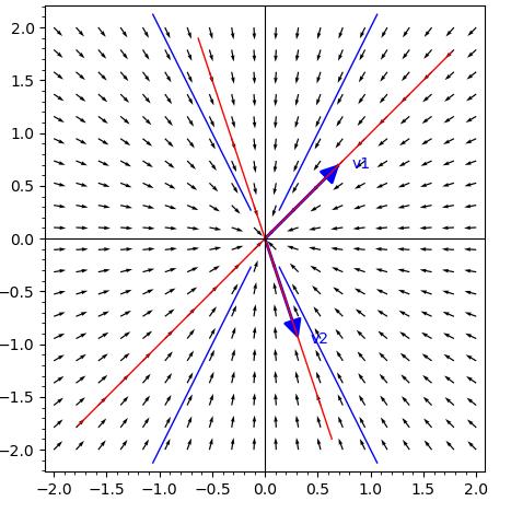
Case 5:\(A\) has a positive eigenvalue (\(\lambda_1\)) and an eigenvalue equal to zero (\(\lambda_2\)). The eigenvectors are \(\mathbf{v_1}\) and \(\mathbf{v_2}\text{,}\) respectively.
Your book identifies these as parallel lines. In the picture below, \(\lambda_1> 0\) and \(\lambda_2=0\text{.}\) The picture displays a vector field for a system with a positive eigenvalue and a zero eigenvalue. The eigenvectors are included and several solution curves. The solution curves are parallel to the line associated with the eigenvector for the positive eigenvalue and approach the line associated with the eigenvector for the zero eigenvalue.
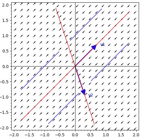
Case 6:\(A\) has a positive eigenvalue of multiplicity 2 (\(\lambda_1 = \lambda_2 > 0\)) that corresponds to two linearly independent eigenvectors are \(\mathbf{v_1}\) and \(\mathbf{v_2}\text{.}\)
This case produces a proper nodal source. In the picture below, \(\lambda_1 = \lambda_2>0\text{.}\) The picture displays a vector field for a system with a single positive eigenvalue that corresponds to two linearly independent eigenvectors. Several solution curves are shown. The solution curves are rays emanating from the origin.
Case 7:\(A\) has a negative eigenvalue of multiplicity 2 (\(\lambda_1 = \lambda_2 < 0\)) that corresponds to two linearly independent eigenvectors are \(\mathbf{v_1}\) and \(\mathbf{v_2}\text{.}\)
This case produces a proper nodal sink. In the picture below, \(\lambda_1 = \lambda_2 < 0\text{.}\) The picture displays a vector field for a system with a single negative eigenvalue that corresponds to two linearly independent eigenvectors. Several solution curves are shown. The solution curves are lines flowing into the origin.
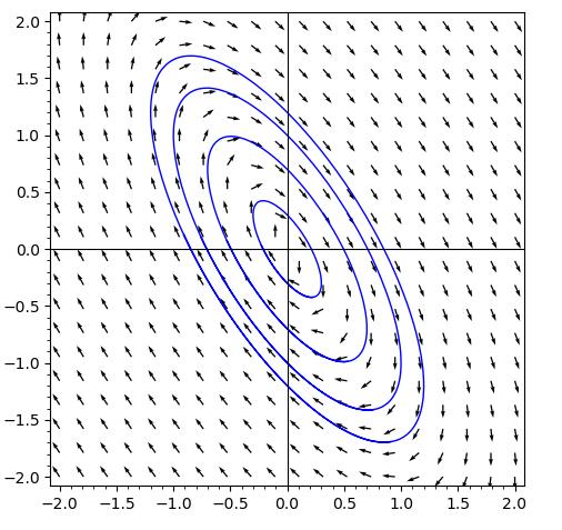
Case 1:\(A\) has purely imaginary eigenvalues (\(\lambda_{1,2} = \pm qi\)) two linearly independent eigenvectors are \(\mathbf{v_{1,2}}=\mathbf{a}\pm\mathbf{b}i\text{.}\)
This case produces a center. In the picture below, \(\lambda_{1,2} = \pm qi\text{.}\) The picture displays a vector field for a system with purely imaginary eigenvalues. Several solution curves are shown. The solution curves are ellipses centered at the origin.
Case 2:\(A\) has complex eigenvalues (\(\lambda_{1,2} = p \pm qi\)) with a positive real part (\(p >0 \)) and two linearly independent eigenvectors are \(\mathbf{v_{1,2}}=\mathbf{a}\pm\mathbf{b}i\text{.}\)
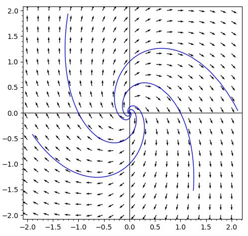
This case produces a spiral source. In the picture below, \(\lambda_{1,2} = p \pm qi\) with \(p>0\text{.}\) The picture displays a vector field for a system with complex eigenvalues that have a positive real part. Several solution curves are shown. The solution curves are spirals emanating from the origin.
Case 3:\(A\) has complex eigenvalues (\(\lambda_{1,2} = p \pm qi\)) with a negative real part (\(p < 0 \)) and two linearly independent eigenvectors are \(\mathbf{v_{1,2}}=\mathbf{a}\pm\mathbf{b}i\text{.}\)
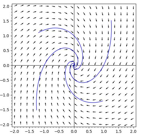
This case produces a spiral sink. In the picture below, \(\lambda_{1,2} = p \pm qi\) with \(p < 0\text{.}\) The picture displays a vector field for a system with complex eigenvalues that have a negative real part. Several solution curves are shown. The solution curves are spirals flowing into the origin.
Case 1:\(A\) has a single positive eigenvalue (\(\lambda_{1,2} = \lambda > 0\)) and only one linearly independent eigenvector. In other words, \(\lambda\) is a defective eigenvalue.
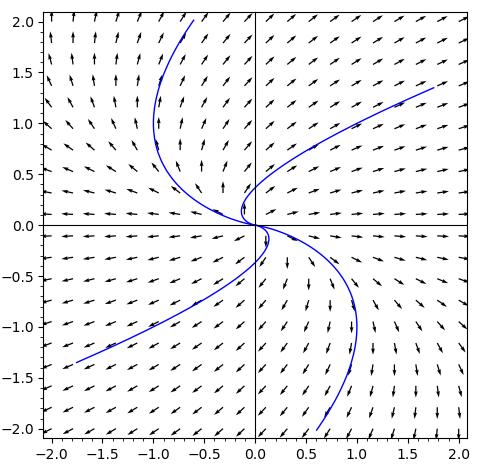
This case produces an improper nodal source. In the picture below, \(\lambda_{1,2} = \lambda >0\text{.}\) The picture displays a vector field for a system with a positive, defective eigenvalue. The solutions curve away from the origin.
Case 2:\(A\) has a single negative eigenvalue (\(\lambda_{1,2} = \lambda < 0\)) and only one linearly independent eigenvector. In other words, \(\lambda\) is a defective eigenvalue.
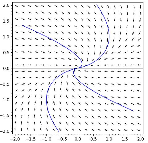
This case produces an improper nodal sink. In the picture below, \(\lambda_{1,2} = \lambda < 0\text{.}\) The picture displays a vector field for a system with a negative, defective eigenvalue. The solutions curve in toward the origin.
Case 3:\(A\) has a single eigenvalue that equals zero (\(\lambda_{1,2} = \lambda = 0\)) and only one linearly independent eigenvector. In other words, zero is defective eigenvalue.
This case produces parallel lines. In the picture below, \(\lambda_{1,2} = \lambda =0\text{.}\) The picture displays a vector field for a system with a zero, defective eigenvalue. It also displays the eigenvector. The solutions are lines that are parallel to the eigenvector. Half of the solutions flow in the direction of the eigenvector and the other half flow in the opposite direction.