Skip to main content
Contents Embed Dark Mode Prev Up Next \( \newcommand{\N}{\mathbb N}
\newcommand{\Z}{\mathbb Z}
\newcommand{\Q}{\mathbb Q}
\newcommand{\R}{\mathbb R}
\newcommand{\set}[1]{\{{#1}\}}
\newcommand{\gint}[1]{\llbracket #1 \rrbracket}
\newcommand{\mean}[1]{\overline{#1}}
\newcommand{\median}[1]{\widetilde{#1}}
\newcommand{\spc}[1]{\underline{\hspace{#1}}}
\newcommand{\del}{\partial}
\newcommand{\intfact}{e^{\int P(x) \, dx}}
\newcommand{\defn}{\stackrel{\textrm{def}}{=}}
\newcommand{\laplace}[1]{\mathscr{L}\set{#1}}
\newcommand{\laplaceinv}[1]{\mathscr{L}^{-1}\set{#1}}
\newcommand{\lt}{<}
\newcommand{\gt}{>}
\newcommand{\amp}{&}
\newcommand{\fillinmath}[1]{\mathchoice{\underline{\displaystyle \phantom{\ \,#1\ \,}}}{\underline{\textstyle \phantom{\ \,#1\ \,}}}{\underline{\scriptstyle \phantom{\ \,#1\ \,}}}{\underline{\scriptscriptstyle\phantom{\ \,#1\ \,}}}}
\)
Handout Lesson 36, Impulses and Delta “Functions”
This lesson is based on Section 7.6 of your textbook by Edwards, Penney, and Calvis.
In our last lesson we used the unit step functions, \(u_a(t)\) to model on/off switches. Today, we will attempt to model sudden bursts such as lightening or hammer strikes. Consider an external force that is only applied momentarily (\(a \leq t \leq b\) ) where \([a,b]\) is a very short interval. The effect of a force often depends only on the impulse \(p\) given by
\begin{gather*}
p=\int_a^b f(t) \, dt
\end{gather*}
Let’s construct a simple function with a unit impulse.
An axis system with a horizontal
\(t\) -axis and a vertical
\(y\) -axis
\(d_{a,\epsilon}(t)=
\begin{cases}
\\
\spc{2.5in} \\
\\
\spc{2.5in} \\
\end{cases}\)
\(\int_a^{a+\epsilon} d_{a,\epsilon}(t) \, dt = \spc{1in} \quad
\text{ for all } a>0, \, \epsilon>0\)
Question What type of "function" would have an
instantaneous unit impulse?
\begin{gather*}
\delta_a(t) = \lim_{\epsilon \rightarrow 0} d_{a,\epsilon}(t) =
\begin{cases} \\ \spc{3in}\\ \\ \spc{3in}\\ \end{cases}
\end{gather*}
Clearly, \(\delta_a\) is not a function in the real numbers. It is sometimes called a generalized function or a distribution.
Definition 248 . Dirac delta function.
\begin{align*}
\delta(t) = \delta_0(t) \defn \begin{cases} \infty \amp
\text{if } t=0 \\ 0 \amp \text{if } t \neq 0 \end{cases}\\
\delta_a(t) = \delta(t-a) \defn \begin{cases} \infty \amp
\text{if } t=a \\ 0 \amp \text{if } t \neq a \end{cases}
\end{align*}
Lemma 249 . Integral property of \(\delta_a(t)\) .
If \(f\) is continuous, then
\begin{gather*}
\int_0^{\infty} \delta_a(t)f(t) \, dt = f(a).
\end{gather*}
\(\mathscr{L}\left\{\delta_c(t)\right\}\) .Number 17 on the table of Laplace transforms gives the following formula:
Theorem 250 .
\begin{gather*}
\mathscr{L}\{\delta(t-c)\} = e^{-cs}
\end{gather*}
Justification:
\begin{align*}
\mathscr{L}\{\delta_c(t)\} \amp = \mathscr{L}\{\delta(t-c)\}\\
\amp = \int_0^{\infty} e^{-st}\delta_c(t) \, dt\\
\amp = e^{-sc}
\end{align*}
Differential equations containing \(\delta_c(t)\) . In this section, we will solve an IVP in which the differential equation contains a
\(\delta\) function.
Example 251 . An IVP with a \(\delta\) function.
Consider the IVP.
\begin{gather}
x''+4x=\delta(t)+\delta(t-\pi) \qquad x(0)=x'(0)=0\tag{#}
\end{gather}
What is the meaning of the right-hand side of the differential equation in this IVP?
What would a solution
\(x(t)\) of
(#) mean?
More workspace on the next page
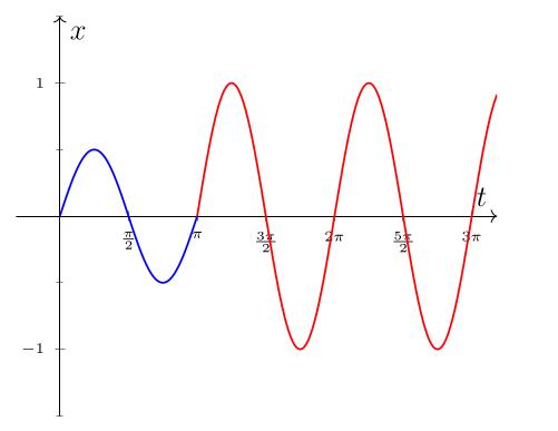
The graph of the solution is shown below
On
\([0,\pi]\text{,}\) the graph is a sine function with period
\(\pi\) and amplitude
\(\frac{1}{2}\text{.}\) On
\((\pi,\infty)\text{,}\) the graph is a sine function with period
\(\pi\) and amplitude
\(1\text{.}\)
Transfer Functions and Weight Functions.
Consider the initial value problem
\begin{gather}
ax''+bx'+cx=f(t) \qquad x(0)=x'(0)=0\tag{#}
\end{gather}
If we apply the Laplace transform to both sides of
(#) , we get
\begin{gather*}
(as^2+bs+c)X(s)=F(s)
\end{gather*}
so
\begin{gather}
X(s) = \frac{F(s)}{as^2+bs+c} = \frac{1}{as^2+bs+c} \cdot F(s)\tag{#}
\end{gather}
Definition 252 .
The
transfer function of the IVP
(#) , denoted
\(W(s)\text{,}\) is given by
\begin{gather*}
W(s) = \frac{1}{as^2+bs+c}.
\end{gather*}
The weight function (or impulse response function ), denoted \(w(t)\text{,}\) is given by
\begin{gather*}
w(t)= \mathscr{L}^{-1}\{W(s)\} =
\mathscr{L}^{-1}\left\{\frac{1}{as^2+bs+c}\right\}.
\end{gather*}
Theorem 253 . Duhamel’s Principle.
The solution of the IVP
\begin{gather*}
ax''+bx'+cx=f(t) \qquad x'(0)=x(0)=0
\end{gather*}
is given by
\begin{gather*}
x(t)=\int_0^t w(u)f(t-u) du.
\end{gather*}
NOTE: Your textbook uses
\(\tau\) instead of
\(u\text{,}\) but I think it is easier to distinguish between
\(u\) and
\(t\) than
\(\tau\) and
\(t\) when you are writing.
Example 254 . Transfer and weight functions.
Find an integral formula for the solution of the IVP.
\begin{gather*}
x''+6x'+9x=f(t) \qquad x(0)=x'(0)=0
\end{gather*}