Lesson 31, Laplace Transformations and Inverse Laplace Transformations

Print preview

Additional printing options

Highlight workspace

Handout Lesson 31, Laplace Transformations and Inverse Laplace Transformations

Textbook Section(s).

🔗

This lesson is based on Section 7.1 of your textbook by Edwards, Penney, and Calvis.

🔗

Section 3 on Trefor Bazett’s website is also a good reference for Laplace transforms.

🔗

The Big Picture.

🔗

We have seen function operators before, namely the \(D^n\) operators.

🔗

\(f(x)\) enters the \(D^n\) operator which produces \(f^{(n)}(x)\)

🔗

Both the and the of the operator are functions.

🔗

Today, we will introduce a new operator: the Laplace Transform, \(\mathscr{L}\text{.}\)

🔗

\(f(t)\) enters the Laplace transform operator \(\mathscr{L}\) operator which produces \(F(s)\)

🔗

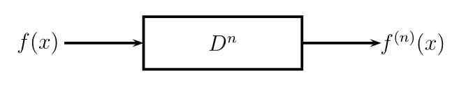
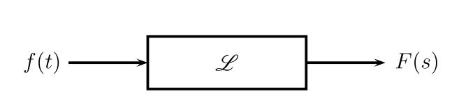
Notice that with the differential operator both the input and the output are functions of the same variable, \(x\text{.}\) With the Laplace transform operator:

🔗

The input function is a function of , which usually represents .

🔗
The output function is a function of , which usually represents .

🔗

With the Laplace transform operator, it is standard to use a letter to represent the input function and its corresponding letter to represent the output function. Why are we studying Laplace transforms in this class? Here is what we hope to be able to do:

🔗

Apply \(\mathscr{L}\) to both sides of a differential equation. This converts our in \(x(t)\) into an in \(X(s)\text{.}\)

A differential equation in \(x(t)\) enters the Laplace transform operator \(\mathscr{L}\) operator which produces and Algebraic equation in \(X(s)\)
🔗

🔗
Next we will open our toolbox and hopefully use algebraic techniques to solve for \(X(s)\text{.}\)

🔗
Finally, we hope to use to find .

🔗

The above strategy does not work for all differential equations, but it is often helpful for differential equations that involve functions with .

🔗

Laplace Transforms.

🔗

Definition 197.

Let \(f(t)\) be defined for all \(t \geq 0\text{.}\) The Laplace transform of f, denoted \(\mathscr{L}\{f(t)\}\) or \(F(s)\text{,}\) is

\begin{gather} F(s) = \mathscr{L}\{f(t)\} \defn \int_0^{\infty} e^{-st}f(t) \, dt\tag{#} \end{gather}

for all values of \(s\) for which the righthand side of (#) converges.

🔗

Example 198. Using the definition of the Laplace transform.

Use the definition of the Laplace transform to find \(\mathscr{L}\{e^{6t}\}\text{.}\)

🔗

Example 199. Using the definition of the Laplace transform.

Use the definition of the Laplace transform to find \(\mathscr{L}\{e^{t^2}\}\text{.}\)

🔗

We mentioned earlier that Laplace transforms are often helpful for solving differential equations when the function has a discontinuity. One way to introduce a discontinuity into a function is to multiply by a unit step function.

🔗

Definition 200.

The Heavyside function, denoted \(u(t)\text{,}\) is defined by

\begin{align*} u(t)\defn \begin{cases} 1, \amp \text{if } t \geq 0 \\ 0, \amp \text{if } t \lt 0 \end{cases} \end{align*}

A unit step function is a horizontal shift of the Heavyside function. More specifically, the unit step function with shift \(c\text{,}\) denoted \(u_c(t)\text{,}\) is given by

\begin{align*} u_c(t)\defn u(t-c) = \begin{cases} 1, \amp \text{if } t \geq c \\ 0, \amp \text{if } t \lt c \end{cases} \end{align*}

🔗

Example 201. Laplace transforms of unit step functions.

Use the definition of the Laplace transform to find \(\mathscr{L}\{u_c(t)\}\text{.}\)

🔗

Table of Laplace Transforms.

🔗

A table similar to the following will be given to you on the final exam.

🔗

Table 202. Laplace Transform Pairs

🔗

#	\(f(t) = \mathcal{L}^{-1}\{F(s)\}\)	\(F(s) = \mathcal{L}\{f(t)\}\)
1.	1	\(\frac{1}{s}\text{,}\) \(s>0\)
2.	\(e^{at}\)	\(\frac{1}{s-a}\text{,}\) \(s>a\)
3.	\(t^{n}\text{,}\) \(n=\) positive integer	\(\frac{n!}{s^{n+1}}\text{,}\) \(s>0\)
4.	\(t^{p}\text{,}\) \(p>-1\)	\(\frac{\Gamma(p+1)}{s^{p+1}}\text{,}\) \(s>0\)
5.	\(\sin at\)	\(\frac{a}{s^{2}+a^{2}}\text{,}\) \(s>0\)
6.	\(\cos at\)	\(\frac{s}{s^{2}+a^{2}}\text{,}\) \(s>0\)
7.	\(\sinh at\)	\(\frac{a}{s^{2}-a^{2}}\text{,}\) \(s>\|a\|\)
8.	\(\cosh at\)	\(\frac{s}{s^{2}-a^{2}}\text{,}\) \(s>\|a\|\)
9.	\(e^{at}\sin bt\)	\(\frac{b}{(s-a)^{2}+b^{2}}\text{,}\) \(s>a\)
10.	\(e^{at}\cos bt\)	\(\frac{s-a}{(s-a)^{2}+b^{2}}\text{,}\) \(s>a\)
11.	\(t^{n}e^{at}\text{,}\) \(n=\) positive integer	\(\frac{n!}{(s-a)^{n+1}}\text{,}\) \(s>a\)
12.	\(u(t-c)\)	\(\frac{e^{-cs}}{s}\text{,}\) \(s>0\)
13.	\(u(t-c)f(t-c)\)	\(e^{-cs}F(s)\)
14.	\(e^{ct}f(t)\)	\(F(s-c)\)
15.	\(f(ct)\)	\(\frac{1}{c}F(\frac{s}{c})\text{,}\) \(c>0\)
16.	\(\int_{0}^{t}f(t-\tau)g(\tau)d\tau\)	\(F(s)G(s)\)
17.	\(\delta(t-c)\)	\(e^{-cs}\)
18.	\(f^{(n)}(t)\)	\(s^{n}F(s)-s^{n-1}f(0)-\dots-f^{(n-1)}(0)\)
19.	\(t^{n}f(t)\)	\((-1)^{n}F^{(n)}(s)\)

Today, we will use numbers 1-12.

🔗

Gamma Function.

🔗

Number 4 on the Laplace transform table uses the Gamma function, \(\Gamma\text{.}\)

🔗

Definition 203.

The Gamma function, denoted \(\Gamma\) is defined as follows:

\begin{gather*} \Gamma(x) \defn \int_0^{\infty} e^{-t}t^{x-1} \, dx \end{gather*}

🔗

Theorem 204. Properties of the Gamma function.

For any \(x \gt 1\text{,}\) \(\Gamma(x)=(x-1)\Gamma(x-1)\text{.}\) (\(x\) need not be an integer for this property.)

🔗
\(\displaystyle \Gamma(1)=1\)

🔗
For any positive integer \(n\text{,}\) \(\Gamma(n)=(n-1)!\text{.}\)

🔗
\(\Gamma\left(\frac{1}{2}\right)=\sqrt{\pi}\text{.}\)

🔗

🔗

Example 205. Computing Gamma function.

Calculate \(\Gamma\left(\frac{3}{2} \right)\text{.}\)

🔗

Properties of \(\mathscr{L}\).

🔗

1. Linearity

The following is Theorem 1 in Section 7.1 of your textbook by Edwards, et.al.

🔗

Theorem 206. Linearity of \(\mathscr{L}\).

If \(a\) and \(b\) are constants, the

\begin{align*} \mathscr{L}\{af(t)+bg(t)\} \amp = a\mathscr{L}\{f(t)\} + b\mathscr{L}\{g(t)\}\\ \amp = aF(s)+bG(s) \end{align*}

where \(F\) and \(G\) exist.

🔗

Example 207. Linearity of \(\mathscr{L}\).

Calculate \(\laplace{\sin^2(5t)}\text{.}\)

🔗

2. Existence

Definition 208.

The function \(f\) is piecewise continous on \([a,b]\) if there are only finitely many discontinuities in \((a,b)\) and they are all jump discontinuities. The function \(f\) is piecewise continous on \([a,\infty)\) if \(f\) is piecewise continuous on \([0,N]\) for all \(N \gt 0\text{.}\)

🔗

Definition 209.

The function \(f\) is of exponential order as \(t \rightarrow \infty\) if there are nonnegative constants \(M\text{,}\) \(c\text{,}\) and \(T\) such that \(|f(t)| \leq Me^{ct}\) for all \(t \geq T\text{.}\)

🔗

Lemma 210.

\begin{equation*} \lim_{t \rightarrow \infty} \frac{f(t)}{e^{ct}} \end{equation*}

equals a finite number, then \(f\) is of exponential order as \(t \rightarrow \infty\text{.}\)

🔗

By this lemma are of exponential order.

🔗

The following is Theorem 2 and its corollary in Section 7.1 of your textbook by Edwards, et.al.

🔗

Theorem 211.

If \(f\) is piecewise continous on \([0, \infty)\) and of exponential order as \(t \rightarrow \infty\) (with constant \(c\)), then the Laplace transform \(F(s)=\laplace{f(t)}\) exists for all \(s \gt c\text{,}\) and \(\lim_{s\rightarrow \infty} F(s)=0\text{.}\)

🔗

3. Uniqueness

🔗

The following is Theorem 3 in Section 7.1 of your textbook by Edwards, et.al.

🔗

Theorem 212.

Let \(f(t)\) and \(g(t)\) be piecewise continous on \([0, \infty)\) and of exponential order. Let \(F(s)\) and \(G(s)\) be their respective Laplace transforms. If there is a constant \(k\) such that

\begin{equation*} F(s)=G(s) \text{ for all } s \gt k \end{equation*}

then

\begin{equation*} f(t)=g(t) \end{equation*}

for all \(t \in [0,\infty)\) where both \(f\) and \(g\) are continous.

🔗

Inverse Laplace Transforms.

🔗

Definition 213.

If \(F(s)=\laplace{f(t)}\text{,}\) then \(\laplaceinv{F(s)} \defn f(t)\text{.}\)

🔗

Example 214. Inverse Laplace transforms.

Evaluate \(\laplaceinv{\frac{s}{s^2-9}}\text{.}\)

🔗

Theorem 215. Linearity of \(\mathscr{L}^{-1}\).